Working Papers explore the
technical and scientific themes that underpin GNSS programs and
applications. This regular column is coordinated by Prof. Dr.-Ing. Günter Hein, head of Europe’s Galileo Operations and Evolution.
Working Papers explore the
technical and scientific themes that underpin GNSS programs and
applications. This regular column is coordinated by Prof. Dr.-Ing. Günter Hein, head of Europe’s Galileo Operations and Evolution.
Peformance analysis of GNSS signal properties and components is well defined in the technical literature. Terms such as code tracking noise, multipath error envelopes, and S-curve bias, to name a few, are commonly accepted and widely used by scientists. However, the performance of GNSS data messages has yet to be fully assessed and compared. This article proposes well-defined “figures of merit” that can be used to better evaluate current and future GNSS system performance and presents sample analyses to demonstrate the authors’ methodology.
The navigation message is an essential part of the navigation signals transmitted by GNSS satellites. The various message formats provide user equipment with all the data needed to compute position-velocity-time (PVT) solutions, to aid various receiver tasks, and to improve positioning accuracy.
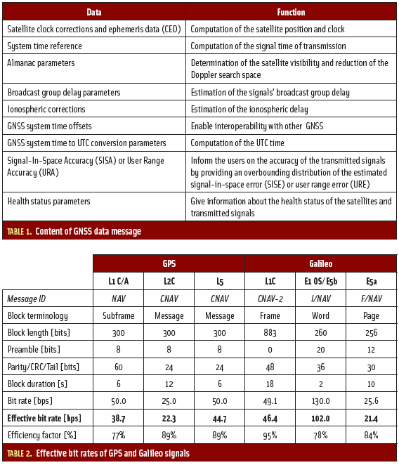
Table 1 (see inset, above right) summarizes the typical content of a GNSS data message.
In some cases, the traditional navigation content is extended to include other data providing additional services. For example the I/NAV message of Galileo will provide search and rescue (SAR) emergency terminals with return link data generated by the rescue centers and transmitted to the Galileo Mission Control Center.
The articles by M. Paonni et alia and M. Anghileri et alia (2010) cited in the Additional Resources, focused on two aspects that are well-known and commonly used in the literature to assess the message performance, namely, the robustness against transmission errors and the time required to retrieve a given set of data from the GNSS signal. The work presented here completes those analyses by extending, redefining, or adding some figures of merit.
In particular we will show that, because some of these terms are closely related to each other, the provided results are more representative of what really happens in the operation of GNSS receivers. We begin by introducing the identified performance dimensions, the related figures of merit, and the methodology used for their computation. The latter portion of the article then compares various GPS and Galileo messages, identifying and demonstrating the strengths and weaknesses of the various message design choices.
Message Performance Dimensions
Four main dimensions have been identified for the characterization of the performance of GNSS data messages: capacity, accuracy, robustness, and timeliness. While accuracy is directly related to the content of the message, the other three factors are related to other properties of the signal carrying the data. We will see that these factors also depend mainly on the design of the message.
Capacity refers to the ability of the signal to transmit useful content to the users and measures the effective amount of data transmitted per time unit. The figure of merit associated with capacity is the effective bit rate, obtained as the average amount of useful information — that is, without overhead, parity, or cyclic redundancy check (CRC) bits — transmitted in one second. In comparing the various GNSS message performance, we present this figure of merit with an associated efficiency factor in percentage terms.
The second dimension considered is accuracy, which refers to the quality of the transmitted information. Most of the content in a GNSS data message consists of parameters representing a certain quantity within the binary-point scaling format. This format represents real numbers with various digits as the multiplication of a signed or unsigned integer value by a scale factor, generally a specific power of two. While the number of bits allocated for a particular parameter gives its range, the scale factor indicates the parameter resolution. Both range and resolution determine the accuracy with which the quantity is provided to users.
The term robustness refers to the capability to provide the users with correct information even if the received data symbols are affected by transmission errors. The figure of merit commonly used to assess this performance dimension is the data demodulation threshold. This is generally defined as the carrier-to-noise ratio (C/N0) of the received signal required to obtain the information bits with an error probability that is lower than a predefined threshold.
The last, but also the most important, performance dimension considered is timeliness, i.e., the capability to provide users with the data they need within a specified time interval. Discussion in M. Anghileri (2010) defined the receiver time to first fix (TTFF) as the sum of discrete contributions related to various receiver tasks that are performed sequentially. The article then emphasized that, in cases where the satellite clock and ephemeris data are not already available at the receiver start, the biggest contribution to the TTFF is the time required to access these data in the navigation message.
The figure of merit computed for assessing the message timeliness is the TTFF-data, defined as the time required by the receiver to access the data needed for the computation of the first position fix (satellite clock and ephemeris data plus the system time reference), starting from the epoch at which the first data symbol can be extracted from the tracking loops.
Comparing Performance of GPS and Galileo Messages
Keeping in mind the definitions of the message performance factors, we now turn to the methodology used for calculating the various figures of merit for capacity, robustness, and timeliness. This same methodology will then be used to assess the performance of the currently available open service GPS and Galileo signals as well as the upcoming GPS L1C.
Capacity. We start with the effective bit rate used to assess capacity. We first identify the amount of bits that are not carrying any useful information but only have some function related either to frame synchronization or to the detection and correction of transmission errors. As shown in Table 2 (see inset, above right), the bits excluded from our computation are the preamble sequences used for frame synchronization purposes, parity bits, CRC bits, and tail bits.
The computation takes into account the fact that most of the messages present different structures. Where the message is structured as a simple repetition of unit blocks that share a common scheme for the ancillary data just mentioned, the unit blocks themselves have been considered for the computation (e.g., NAV subframe, CNAV messages, F/NAV pages).
If the unit blocks presented some differences, relevant for calculating the effective bit rate, we considered a higher level block of data repeating with the same structure (e.g., frames instead of subframes for GPS CNAV-2 computation, words instead of pages for Galileo I/NAV).
Parity bits are used in the GPS NAV (6×10 bits) message, while the CRC-24 is used in all other messages. Note that only two out of three subframes of L1C have CRC (total of 48 bits). Galileo signals are the only ones using tail bits to improve the decoding performance of the convolutional codes.
In particular, six tail bits are used in each page, resulting in 12 tail bits for the I/NAV two-page word and six tail bits for the F/NAV page. In the I/NAV computation, two synchronization patterns of 10 bits belonging to the even and odd pages, respectively, are considered part of the ancillary data and therefore do not contribute to the effective content.
The GPS L1 C/A, L5 and L1C signals present almost the same bit rate. However, the effective bit rate of the NAV message is significantly influenced by the high number of parity bits. (This message has no other error protection scheme.)
The GPS L2C and Galileo E5a signals are very similar in terms of bit rate and effective bit rate, even if a shorter preamble and the absence of the tail bits make the CNAV of L2C a little more efficient. However, thanks to these differences the F/NAV has better synchronization properties and decoding performance.
The most significant indication obtained with this figure is the very high bit rate at which the Galileo I/NAV message is transmitted. This design choice was mainly driven by the requirement of the timely provision of the large amount of integrity data foreseen for the original Galileo Safety-of-Life service. However, as we will see next, this advantage in terms of high bit rate cannot be properly exploited for navigation purposes by Galileo users: on the one hand, more than half of the I/NAV message does not contain data that is directly used for navigation, and on the other hand, the high bit rate penalizes the message robustness.
The innovative message structure of CNAV-2 — the fact that the error correcting codes used (BCH and low-density parity-check, LDPC) do not need tail bits and the additional feature that frame synchronization is performed by correlation with the overlay code modulated on the pilot channel — bring the efficiency factor of GPS L1C to 95 percent, which is better than any other signal.
For the scope of this work, we limit the assessment of the accuracy of the various navigation messages to the satellite clock and ephemeris parameters that indeed represent the core of the navigation data content. Table 3 compares the number of allocated bits and the associated scale factors for the satellite ephemeris parameters in various GPS and Galileo messages.
First of all, the satellite ephemerides of the GPS NAV message and those of Galileo present the same range and resolution, i.e., the same accuracy according to the definition we have given earlier. Note that the real accuracy of the ephemeris also heavily depends on the orbit determination and time synchronization (ODTS) performance of the respective ground segments.
The CNAV and CNAV-2 messages present various differences: for almost every parameter the resolution was improved (smaller scale factors), some ranges were reduced, and for some parameters a different dissemination strategy was chosen. In particular, for the semi-major axis and for the mean motion, first-order effects are taken into account by transmitting two additional parameters: adot and Δndot.
Furthermore, by transmitting delta values to fixed reference values (e.g., Δa with respect to aref = 26,559,710 meters, as specified in the GPS L1C interface specification document), the number of bits used could be reduced and, at the same time, the resolution could be improved. These changes brought an 18 percent increase for CNAV and CNAV-2 in the amount of data allocated to the satellite ephemerides with respect to the other navigation messages.
Looking at the satellite clock correction parameters, shown in Table 4, we can see that the modernization of the GPS message brought improvements in the resolution of the parameters and modified the ranges for the first- and second-term polynomial coefficients. Unlike the ephemeris parameters, the clock corrections of Galileo present higher ranges and better resolution than those transmitted in the GPS NAV message.
Message Robustness. We will now focus on the methodology for the assessment of the message robustness. Unlike communication systems in which bit errors could simply bring about a still-acceptable lower quality of service, navigation data can only be used if they are free of errors. To ensure this, the data bits are arranged into blocks, and specific check techniques (e.g., CRC) are used to validate the error-free condition.
Therefore, the error probability to be considered for the assessment of the message robustness should be in terms of block error rate and not in terms of bit error rate. To improve robustness, Galileo and modernized GPS incorporated more advanced techniques, including forward error correction (FEC) and block interleaving, into their navigation messages.
Navigation messages are generally broadcast with a more or less fixed repeating pattern, such that the content is provided to users with a certain repetition rate. As explained earlier, if a specific data block contains some errors, the receiver will discard it and simply wait for the next repetition of that data.
Although this signal processing design is generally not problematic for most data content, losing part of the data required for the first position fix can significantly increase the receiver TTFF and disappoint users, especially in the mass market sector. Therefore, instead of comparing the message robustness for a generic unit block, we propose to focus the assessment on the most sensitive parts of the message, namely the satellite clock correction and ephemeris data (CED).
This method assesses message robustness by computing the data demodulation threshold. In our work, this will be specifically applied to the parts of the navigation message containing the CED.
The robustness of a GNSS data message depends on many factors:
1. minimum received signal power level
2. amount of power dedicated to the data channel (possible split with pilot)
3. symbol rate of the signal
4. error protection techniques employed (FEC, interleaving)
5. channel conditions.
The first factor simply expresses the fact that signals received with higher minimum power levels have a better margin to the data demodulation threshold, while all other factors are directly influencing the threshold value. The second factor takes into account that the amount of power effectively available for the data channel might be lower than that of the overall signal, for example, if the power is shared with a pilot component (all signals except L1 C/A). The third factor can be understood with the help of Equation (1).
The energy per symbol to noise density ratio (ES/N0), which also represents the signal-to-noise ratio (SNR) of the signal, is given by multiplying the C/N0 of the signal by the inverse of its symbol rate, i.e., by the symbol duration. The higher this energy is, the lower the probability that the demodulated data will be affected by errors. For the same received C/N0, the signal transmitted at the lower rate will present a lower error probability.
In terms of the data demodulation threshold, this translates into Equation (2).
For signals showing the same ES/N0 threshold, the signals transmitted at lower data rates will show a lower C/N0 threshold.
Factors four and five are related to each other in the sense that the error correction performance of the employed protection technique shows a different behavior in the additive white Gaussian noise (AWGN) channel and in more realistic channel models. The following robustness assessment takes all these points into account and discusses in detail their effects on the final results. Table 5 summarizes the information related to the first four factors for the GPS and Galileo signals under analysis.
Because many signals present different error protection techniques, the first result we show has the goal of comparing their correction performance independent of the data rate of the signals and of the block lengths. For this reason, the results are a function of the ES/N0 and not of the C/N0. We applied the convolutional codes of GPS and Galileo to blocks of length 600 and compared the results with the threshold obtained with the LDPC codes used for the GPS L1C Subframe 2 of the same length.
Figure 1 shows the obtained curves: in particular the benefits of using tail bits (main difference between the GPS and Galileo convolutional codes, CCs) and the coding gain brought by the LDPC codes are clearly visible.
Since both types of FEC (convolutional and LDPC) have a coding rate of one-half while the BCH codes applied to the GPS L1C Subframe 1 use a much higher redundancy (9/52), the comparison among them would be not fair. However, the curve of the BCH codes has been included in the figure to give an indication of the coding gain provided by these codes.
The error correction capability of the Hamming codes used to protect the GPS NAV message is very limited and the associated error curve, also present in Figure 1 for reference, is very close to that of the uncoded BPSK modulation. The benefit brought by the block interleavers will be shown later together with the results obtained in the land mobile satellite (LMS) channel, where burst errors are more likely to occur.
Further significant differences among the signals are given by the last three rows of Table 5. A 50 percent power allocation to the data component will translate into a –3-decibel difference with respect to GPS L1 C/A, which has no pilot component, while for L1C this difference will be –6 decibels. This produces a corresponding effect on the value obtained for the data demodulation threshold.
In the same way, as explained earlier, signals presenting a symbol rate that is twice (GPS L5, L1C) or five times (Galileo E1/E5b) higher than 50 sps will be penalized by 3 and 7 decibels, respectively. Finally, the differences in the minimum received power level must also be considered when drawing conclusions on the robustness of the different messages, because a difference of up to 4.5 decibels is present across the various signals (e.g., GPS L1C/A or L2C versus GPS L5).
In order to be as representative as possible of real use cases for applications in urban and suburban scenarios, we included a specific two-state LMS model for the analysis described in the article by Prieto-Cerdeira et alia (Additional Resources) in addition to the AWGN channel, which is widely accepted for modeling open sky scenarios without strong multipath components.
This LMS model includes the effects of multipath, resulting in Doppler frequency dispersions of the received signal, as well as shadowing or blockage effects due to the particular environment in which the signal is received. For convenience, the model terms the two states as “Good” and “Bad,” respectively representing a range of line-of-sight-to-moderate shadowing and moderate-to-deep shadowing.
For assessing the performance of the GNSS messages considered in this research, we used the channel configuration shown in Table 6. Indeed, this challenging configuration enables us to better see the benefits of the various FEC and interleaving schemes.
Figure 2 shows the amplitude and the phase of the channel coefficients obtained with the implemented LMS model. The two states are clearly visible, with very strong attenuation effects (down to –50 decibels) appearing in the “Bad” state for this scenario configuration.
Figure 3 presents the simulation results obtained in the AWGN channel.
The data demodulation thresholds were computed by intersecting the CED error rate curves obtained by Monte Carlo simulations with a threshold value equal to 10-2. This means that, if during the considered simulation time the received signal has an average C/N0 equal to or bigger than the computed threshold, the CED will be correctly decoded at least 99 times out of 100. Table 7 summarizes the obtained thresholds.
GPS L2C and Galileo E5a deliver the best performance mainly because of their very low data rate, with the Galileo signal also exploiting the advantage of using tail bits to help the decoding process. Next in line for performance we find the GPS L1C, despite the fact that only 25 percent of the power is allocated to the data channel.
Here, the coding gain of the LDPC codes plays an important role. The GPS L5 signal presents a threshold exactly 3 decibels higher than L2C, because of the doubled data rate, but we should also remember that its minimum received power is 4.5 decibels higher.
The same reason (high data rate) explains the poor performance of the Galileo E1-OS signal: the 7 decibels of disadvantage with respect to the GPS L1 C/A code transmitted at 50 symbols per second is only partially recovered by the presence of FEC. The results of the analysis in the LMS channel are shown in Figure 4 and Table 8.
The effects of multipath, fading, and also total signal obstruction, which characterize the simulated urban environment, resulted in the significant increase of the data demodulation thresholds, as can be seen in Table 8. GPS L1 C/A has the worst robustness in this case because it lacks any FEC or interleaving techniques. The presence of block interleaving in the Galileo E1-OS signal also explains the improved performance with respect to the GPS L2C and L5 signals, visible in Figure 4.
As expected, the effectiveness of the LDPC codes used for protecting the GPS L1C signal is even more evident in the LMS channel and gives almost the best performance, despite the lower amount of power allocated to the data component. Galileo E5a is confirmed to have the best robustness, mainly due to the combination of low data rate, long interleaved blocks, and well-terminated convolutional codes.
Timeliness. We now turn to the methodology for assessing navigation message timeliness. The figure of merit to be computed is the TTFF-data (TTFFD), namely the contribution to the total TTFF deriving from the collection of the data required for the first position fix.
In estimating the TTFFD, we first identify the location of the first-fix-data in the navigation message pattern, marking which data blocks contain the satellite ephemeris and clock correction parameters and the counters associated with the GNSS system time. An example of this first step is given in Figure 5, where the location of the first-fix-data in the I/NAV words transmitted on the Galileo E1-OS signal is shown. The clock and ephemeris data (CED) are distributed over four different words (Types 1-4). In order to use the data contained in these four blocks the receiver must retrieve a valid version of each of them.
The “TOW” counter present in the word types 5, 6, and “spare” stands for Time-of-Week and gives the system time of transmission at the beginning of the word containing it in terms of seconds elapsed since the start of the current week. The information about the system time reference can be gained as soon as one of these blocks has been correctly decoded.
To understand the second step of the computation, imagine a GNSS user turning on a receiver at a certain epoch. After acquiring the signal and then switching to the tracking mode, the receiver extracts navigation data. The first available data symbol will be located in a position uniformly distributed within the word pattern (e.g., I/NAV subframe).
Depending on its status, before being able to perform the first position fix, the receiver needs to retrieve the first-fix-data from at least four satellites. For the scope of our analysis, we assumed that the computed TTFFD refers to the worst of the first four satellites being used for the position solution. The TTFFD will be the time elapsed between the epoch at which the first data symbol is extracted from the received signal and the epoch at which the entire set of first-fix-data is obtained.
If all possible data transmission errors due to the presence of the channel can be corrected at the receiver, for a given message structure characterized by a certain amount of data symbols sent at a certain repetition rate the TTFFD is simply a function of the entry point in the data block pattern (e.g., 30-second subframe for Galileo I/NAV). On the other hand, if after the message decoding some errors remain, the currently processed data block must be discarded and its content cannot be accessed until the next transmission.
The computation of the TTFFD was carried out with a software tool simulating the end-to-end transmission of GNSS messages at symbol level. For modeling the transmission channel, both AWGN and the LMS model described previously were used. In this way, we can take into account the influence of the real message structure, of the error correction techniques employed, and of other signal parameters, such as the data rate or the amount of power allocated to the data channel.
An example of TTFFD computation results is given in Figure 6, where the TTFFD of a receiver processing the Galileo E1-OS signal is shown for the case when the received data was error-free.
The minimum value for the TTFFD (14 seconds) is obtained when the first symbol available is right at the beginning of Word Type 1 (see Figure 5), which is located 20 seconds after the beginning of the subframe. If this first symbol is skipped, then the TTFFD jumps up to the maximum value (32 seconds) because the receiver must wait for the current incomplete word (about 2 seconds) plus one complete subframe (30 seconds).
If the content of a certain word is not relevant in terms of TTFFD, skipping the first symbols has no effect on the final result. Indeed, starting from the epochs at 2 seconds or 22 seconds, the curve only decreases. Skipping the first symbol of a word type containing the system time reference does not produce the same jumps as for the CED. This can be explained by the fact that the subframe contains more than one repetition of the “TOW” counter.
Once the TTFFD function has been obtained, three different indicators are defined to better characterize the analysis and also allow comparisons among different signals: TTFFDavg, TTFFDworst, and TTFFD95.The first two indicators simply represent the average and the highest value that the TTFFD assumes over the whole subframe and are equal to 25.4 seconds and 32.0 seconds, respectively. The third indicator, TTFFD95, gives the value with a 95 percent confidence and is generally considered the most significant indicator.
To obtain TTFFD95, one has to compute the associated probability density function (PDF). Next, Equation (3), representing the cumulative distribution function, must be solved for the variable TTFFD.
In the equation, f(t) represents the PDF of the TTFFD. Figure 7 and Figure 8 show the PDF and CDF, respectively, of the computed Galileo E1-OS TTFFD.
In particular, the CDF curve can be used as a figure of merit for comparing the TTFFD performance of the GPS and Galileo signals. The accompanying figures illustrate the effect of the presence of some bit errors in the first-fix-data blocks of the received subframe. The signal transmission was simulated in the same urban environment used for the robustness assessment. In this case, the statistics were computed with an LMS channel realization of 20 minutes, simulating the message end-to-end transmission for all the possible receiver switch-on epochs (with one-second resolution).
Looking at the TTFFD curve in Figure 9, one can see that whenever the bit errors affected a part of the I/NAV subframe containing the clock and ephemeris data, the receiver had to wait for the next repetition and the curve showed jumps of 30 seconds, i.e., the duration of an entire subframe. The presence of bit errors and their effect on the TTFFD is also clearly visible in the PDF and CDF curves, as shown in Figure 10 and Figure 11, respectively.
We compare the TTFFD performance of the GPS and Galileo signals considered in the previous robustness analysis by showing the numerical results of the TTFFD computation and the various cumulative distribution functions (CDFs). Table 9 and Figure 12 summarize the results of the TTFFD computation in the AWGN channel with high line-of-sight (LOS) C/N0, a condition sufficient to avoid the presence of bit errors in the received data.
Looking at the results, we can see that the main factor affecting the results is the maximum broadcast interval between two CED sets. In particular, the GPS L1C signal shows a very short TTFFD value (18 seconds). This is understandable considering the possibility of combining the data from different frames in the navigation message. In fact, the overlay code on its pilot component and the fact that the CED remains constant over a fixed amount of time (two hours) allow for this combination.
Galileo E1-OS and E5b are heavily penalized by the large amount of additional content transmitted within the 30-second subframe (also giving that particular slope to the CDF curve), while other signals generally perform worse than these because of the lower data rates. Table 10 and Figure 13 show the results obtained in the LMS channel and enable us to complete the analysis, taking into account the message robustness of the different signals.
Comparing the CDF curves obtained in the LMS channel with those obtained in the AWGN channel, we can see that the performance ranking of the various signals is maintained, with the exception of the GPS L1 C/A code. In fact, its robustness is known to be critical since no FEC is used. Signals transmitted at low data rate (L2C and E5a) show strong robustness, with the Galileo signal taking advantage of the presence of the block interleaver.
Galileo signals carrying the I/NAV message have the disadvantage of a high data rate, which negatively affects the message robustness. Sometimes more than one message repetition was needed to obtain correct data. The GPS L1C signal demonstrates the best TTFFD performance. Indeed, its message robustness — achieved from the combination of long interleaved blocks, advanced FEC (LDPC codes), and moderate data — rate gives it a substantial advantage over the other signals.
Conclusions
Starting from the need for a clearer and more extensive methodology for the assessment of GNSS data message performance, this article identified four fundamental dimensions: capacity, accuracy, robustness, and timeliness. The GPS L1C signal almost always gives the best performance in terms of accuracy, robustness (second only to Galileo E5a), and timeliness. The great potential of the Galileo E1-OS/E5b signals in terms of high capacity cannot be properly exploited due to the presence of a large amount of reserved data and currently only reflects the associated limitation in terms of message robustness.
The analysis proved that the key factors for good data-delivery performance cannot be identified separately but should instead be considered through figures of merit that are able to combine the effects of the message robustness and its timeliness.
In view of future GNSS signal and message design activities, especially if these efforts are targeting the optimization of the signal performance in terms of robustness and TTFF, the following recommendations can be made:
- Limit the data content to navigation data or clearly separate data for additional services in order to be able to guarantee high repetition rates for the first-fix-data.
- In the trade-off of robustness versus TTFF, keep the data transmission rate as low as possible, as this heavily impacts the message robustness. This could be possible if the previous recommendation to limit data content is heeded.
- Use efficient error protection techniques, such as advanced FEC and block interleaving.
- Block durations on the order of some seconds are a good compromise between latency and robustness against fading (note strong performance of GPS L1C and L5).
- Allocate the CED to a specific data block containing only data that could remain invariant over a certain time interval (e.g., one to two hours). This allows for the reception of partial blocks and has a significant positive effect on the TTFFD.
Most of these recommendations clearly reflect the design characteristics of the GPS L1C signal. However, considering future designs, we believe that a further improvement in terms of robustness or bit rate (and thus TTFF) could be achieved, for example, by adopting some more advanced FEC techniques like those reviewed in the article by Anghileri et alia (2011).
Acknowledgements
This article is mainly based upon the work done in the framework of the Ph.D. dissertation of Marco Anghileri and represents a prepublication of some of its main results. The software tools used for the message performance analysis were partially developed in the framework of the ADVISE project, a study funded by the European Space Agency (ESA). Note that the content of the present article reflects solely the authors’ view.
Additional Resources
[1] Anghileri, M. (2010), M. Paonni, S. Wallner, J. A. Avila-Rodrigues, and B. Eissfeller, “Ready to Navigate! A Methodology for the Estimation of the Time-to-First-Fix,” Inside GNSS, March/April 2010
[2] Anghileri M. (2011), and M. Luise, A. Perotti, A. Tarable, M. Paonni, B. Eissfeller, G. López-Risueño, and F. Zanier “A Fresh Look into Designing Channel Error Protection Codes for Satellite Navigation Messages,” Proceedings of the GNSS Signals Workshop, Toulouse, France, 2011
[3] European Union, European GNSS (Galileo) Open Service, Signal In Space Interface Control Document. Version 1.1
[4] GPS Directorate, Navstar GPS Space Segment/User Segment L1C Interface, IS-GPS-200 Rev. F, 2011
[5] Paonni, M., M. Anghileri, J. A. Ávila-Rodríguez, S. Wallner, and B. Eissfeller, “Methodologies for the Determination of the Minimum Required Carrier to Noise Ratio to Receive GNSS Signals,” Proceedings of the 4th European Workshop on GNSS Signals and Signal Processing, Oberpfaffenhofen, Germany, December 2009
[6] Prieto-Cerdeira, R., and F. Perez-Fontan, P. Burzigotti, A. Bolea-Alamañac, and I. Sanchez-Lago,“Versatile Two-State Land Mobile Satellite Channel Model with First Application to DVB-SH Analysis,” International Journal of Satellite Communications and Networking, Volume 28, Issue 5–6, pages 291–315, September-December 2010


