Q: How do measurement errors propagate into GNSS position estimates?
A: Not surprisingly, GNSS positioning accuracy is largely dependent on the level of measurement errors induced by orbital inaccuracies, atmospheric effects, multipath, and noise. This article discusses how, specifically, these errors manifest as position errors.
Estimating a Position
For the purpose of our discussion here, we only consider least-squares estimation with no a priori knowledge of the receiver’s position or time. To this end, least-squares assumes the measurements, ⃗z, are related to the states (position and clock bias, in the case of GNSS), ⃗x, as follows
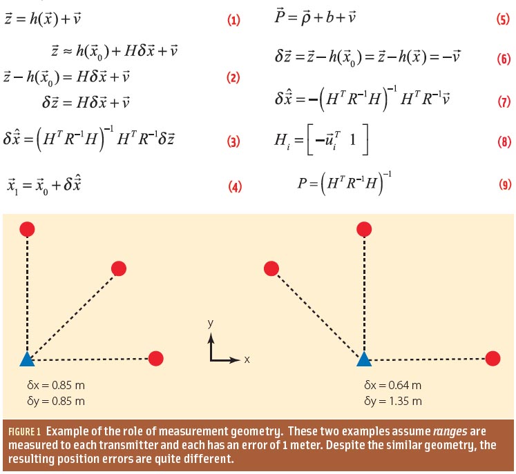
Equation (1) (see inset photo, above right, for all eqautions)
where h(•) is the measurement model — assumed, for convenience, to be non-linear — and (⃗v) is the vector of measurement errors. This equation is linearized to yield
Equation (2)
where ⃗x0 is the current estimate of the state vector (point of expansion), δ⃗x is the error of ⃗x0 relative to the (unknown) true states, H is the Jacobian matrix (also called the design matrix, observation matrix, or geometry matrix), and δ⃗z is the misclosure vector, which is the difference between the true measurements (⃗z) and the measurements estimated from the current states (i.e., h(⃗x0)).
The well-known solution to equation (2) is as follows:
Equation (3)
where R is the covariance matrix of the measurement errors. The initial state estimates are then updated as follows
Equation (4)
Because the model is non-linear, we can use iteration to converge to the final solution.
Role of GNSS Errors
For the purpose of this article, the pseudorange measurement equation (equivalent to equation [1]) is written as
Equation (5)
where ⃗P is the vector of pseudoranges from all satellites in view, ⃗ρ is the vector of geometric distances between the receiver and the satellites, b is the receiver clock error (common across measurements), and ⃗v is the aggregate measurement error from all error sources. Although we aggregate all of measurement errors together, individual components (e.g., troposphere) could be separated and easily worked through the following development.
Let us now consider the specific case where the initial state estimate was perfect such that ⃗x0 = ⃗x. Although this is an unrealistic scenario (if you knew the true position in advance, you do not need GNSS!), it serves as a useful illustration of how measurement errors affect the final solution. Furthermore, since the least-squares approach will yield the same position estimate for all reasonable initial state estimates (in this case, “reasonable” would include a position accurate to at least 1,000 kilometers), this scenario is not limiting.
For the assumed case, the true value of δ⃗x is zero. It follows that if the value estimated from equation (3) differs from zero, this actually represents the error in the estimated states. To obtain a more explicit equation, we first compute the misclosure vector as follows
Equation (6)
In other words, the misclosure vector contains the measurement errors only. Finally, substituting this result into equation (3) gives
Equation (7)
Equation (7) shows how measurement errors propagate into the final solution. Although the equation is relatively simple, there is no hard-and-fast rule for describing how this happens. Rather, we can only say that two key things determine the effect of measurement error on the final solution: the relative measurement accuracy reflected in R, and the measurement geometry as reflected in the Jacobian.
Before looking at these aspects in more detail, note that equation (7) shows the effect on all state estimates separately (i.e., as a vector). This is important because some applications may be more interested in certain parameters than in others. For example, aviation is more sensitive to vertical positioning errors than horizontal positioning errors. In contrast, timing applications are not concerned at all with the position states.
Measurement Accuracy
Intuitively, the more accurate a measurement is assumed to be, the more weight will be given to that measurement. As R is the covariance matrix of the measurement errors, this weighting of the measurements happens “automatically” within the least-squares estimation process.
Of course, because the user (or perhaps software programmer) is responsible for selecting the covariance model, careful decisions need to be made in this regard; otherwise results will be suboptimal.
Measurement Geometry
To further explain the idea of measurement geometry, a single row of the Jacobian matrix (corresponding to the i-th single measurement) can be written as
Equation (8)
where ⃗ui is the unit vector pointing from the receiver to the i-th satellite. The distribution of all satellites relative to the user reflects the measurement geometry. This is often quantified using dilution of precision (DOP) values.
To illustrate the importance of measurement geometry, consider Figure 1 (inset photo, above right), which shows two measurement scenarios for a two-dimensional positioning problem. In both cases, the receiver (blue) is measuring ranges (not pseudoranges) from the transmitters (red). Each transmitter is assumed to have an error of one meter, and all measurements are given equal weight (i.e., same variance).
The distribution of transmitters appears to be relatively similar; only one transmitter is moved (mirrored across the y-axis). Nevertheless, this small difference in measurement geometry results in different position errors.
Similar examples can be developed for the three-dimensional case, but this is more complicated to draw and is omitted here.
Unfortunately, users cannot place satellites to optimize measurement geometry. The best that can be done is to use mission-planning utilities to collect data during parts of the day where geometry is best (in the area of the data collection). Of course, using receivers that track satellites from multiple GNSSs will inherently improve the geometry too.
Estimating Clock Errors
The examples in the previous section only considered the case of measured ranges, meaning the clock error state does not need to be estimated. However, estimating the clock error — which is common across all measurements — can significantly affect results.
In particular, although we name the state the “clock error,” the estimated value will include the true clock error along with anything that appears to be common across all satellites.
With this in mind, if we repeated the previous examples using pseudoranges (thus requiring the clock error to be estimated), the fact that all measurements were assumed to have a one-meter error means that the least-squares estimator could not separate the true clock bias from the common error. The result would be that the clock error estimate would be biased by one meter (in this case), but the position error would actually be zero!
Different Types of Errors
Although equation (7) completely defines the propagation of a specific set of errors (i.e., at a particular instant of time) from the measurement domain to the position (and time) domain, this equation is usually reserved for systematic errors that manifest as biases in the short- or long-term. Such errors would include biases resulting from unmodeled atmospheric effects, satellite orbital errors, and so forth.
Measurement blunders would also be considered systematic errors. In fact, equation (7) is used when assessing the reliability and integrity of a positioning system in the presence of blunders.
Random errors such as multipath and noise, however, are usually treated a bit differently. Specifically, these errors are usually well characterized by their standard deviation only (i.e., no bias), meaning their effect can be completely reflected in the measurement covariance matrix.
If this is the case, the effect of these errors on the solution is directly obtained from the covariance matrix of the estimated parameters, which is computed as
Equation (9)
This is a by-product of the law of propagation of variances. As before the result is affected by the measurement geometry and the measurement accuracy.
Summary
This article looked at how measurement errors propagate into positioning errors. The primary factors affecting this propagation are measurement geometry and the measurement accuracy. This explains the motivation for receivers that minimize measurement errors (especially multipath) and that track as many satellites as possible.


