 Equations 2, 7, 8, 9, 10 & 11
Unmanned aerial vehicles (UAV) are finding increased application in both domestic and governmental applications. Small UAVs (maximum take off weight less than 20 kilograms) comprise the category of the smallest and lightest platforms that also fly at lower altitudes (under less than 150 meters).
Designs for this class of device have focused on creating UAVs that can operate in urban canyons or even inside buildings, fly along hallways, and carry listening and recording devices, transmitters, or miniature TV cameras.
Operational requirements for these kinds of UAVs typically encompass flying close to the ground and in relatively narrow spaces with a lot of obstacles. This introduces problems for a simplistic application of technologies used in larger UAVs. In particular, the rotary wing UAV platforms used in those scenarios provide vertical takeoff and landing and hovering capability, but they are intrinsically unstable systems requiring high-rate and accurate attitude and position data to be automatically controlled.
Automatic control of the degrees of freedom of such flying robots is the key factor to make them easily usable by a trained but not particularly skilled pilot; therefore, it is essential for such devices if intended for a wide commercial market.
Small, lightweight, power-efficient, and low-cost microelectromechanical system (MEMS) inertial sensors and microcontrollers available in the market today help reduce the instability of such platforms making them easier to fly. Current MEMS inertial measurement units (IMUs) come in many shapes, sizes, and costs — depending on the application and performance required — and are widely used as sensors for relative position estimation.
Although MEMS inertial sensors offer affordable, appropriately scaled units, they are not currently capable of meeting UAV requirements for accurate and precise navigation due to their inherent measurement noise. However, the accuracy of a MEMS-based inertial navigation system (INS) can be improved by integrating them with a GNSS receiver, simultaneously developing appropriate integration mechanisms.
This article describes an integrated multi-GNSS/INS system — developed and tested in both a car and on board a small quadrotor — that has been designed to achieve sufficiently accurate position and attitude control using lightweight and ultra low-cost components so as to be suitable for the technological and commercial aspects of the vehicle.
The architecture combines the advantages of absolute satellite-based positioning with the high dynamic performance and data rates of inertial sensors. The article will describe the system architecture, its carrier phase–based methodology for positioning and attitude determination, and an evaluation of the system’s performance of achieved results during real-time tests.
System Architecture Definition
Figure 1 shows a simplified block diagram of the developed on-board unit. The sensor package is composed of four non-professional, non-dedicated commercial-off-the-shelf (COTS) GNSS chipsets connected to one patch antenna each and attached to the tips of an ad hoc cross-shaped structure fixed to the quadrotor body. A motion-grade COTS MEMS IMU placed near the center of mass of the UAV measures angular rates and accelerations.
The main goal of the final system is to achieve a compact and cost-effective real-time position and attitude estimator, which is the reason why the components employed are relatively inexpensive compared to readily available platforms with costlier and bulkier elements. Therefore, an important investment of effort has been made in the system integration and in the development of specific techniques and algorithms to achieve high performance () with the combination of devices of individually moderate accuracy.
These low-cost receivers provide information to the “Processing Unit” (PU) block shown in Figure 1 in the form of so-called raw measurements, that is, basic GNSS signal-in-space data such as pseudoranges or carrier phase readings, in addition to standard position, velocity, and time (PVT) outputs. These outputs, along with the readings produced by the IMU (and possibly other sensors) are processed in the PU by a real-time microprocessor-based platform, which gathers and synchronizes these data and applies the fusion algorithms to compute the PVT and attitude (PVTA) of the platform. This PVTA estimator works on top of the standard vehicle control unit of the UAV.
The system is designed to provide high-accuracy attitude performance based on precise GNSS carrier phase measurements, reducing the position errors by combining measurements from several receivers. Furthermore, the aid of the IMU allows the high data output rate necessary for active attitude control and increases the reliability of the GNSS based attitude solution when its information is used in the ambiguity resolution process.
In the following sections we present an overview of the main functionalities developed within the processing unit, discussing their design principles and the criticisms associated with their practical implementation.
The PVTA Processing Unit
Figure 2 illustrates the architecture of the proposed navigation system (PVTA estimator) and the custom board hosting it, developed by Acorde Technologies, S.A., which is based on an ARM9 microcontroller.
This works at a clock frequency of 400 megahertz, includes two separate data and instruction cache memories of 32 kilobytes each, and two high performance sets of ROM and RAM memories of 64 and 32 kilobytes, respectively. Additionally, the board includes a SDRAM controller to interface external memory, addressable linearly up to 64 megabytes, and allowing back switching with eight-chip selects. Moreover, QNX has been selected as the real-time operating system that offers specific support for this platform and can be easily run on the board without needing to adapt it to the particular hardware setup.
Sensor Synchronization
Low-cost GNSS receivers, IMUs, and other sensors generate data in principle asynchronously with respect to each other. GNSS receivers are expected to be intrinsically synchronized among each other using the internal 1PPS signal (a one-hertz pulse). The GNSS time reference can be considered absolute for sensor synchronization purposes. In our case, this one-hertz reference is also the rate at which the GNSS modules generate observables.
The selected IMU uses its own clock (nominally 100 hertz), providing sensor data samples not aligned with the GNSS time reference or even synchronized, as this internal clock is very low precision. The IMU also generates interrupt requests (IRQ) to notify the PU whenever new inertial measurements are sampled.
Figure 3 depicts the adopted synchronization scheme, which is based on two conceptual modules (the host and the synchronization hardware [SHW]), both residing in the PU. The general time reference is given by the 1PPS signal from the base GNSS receiver, which is followed by all four GNSS modules sending their respective observables to the “host” with a small latency on the order of a few milliseconds. The GNSS data is also used to obtain the integer number of GPS seconds to which the last one-hertz pulse and subsequent carrier/pseudorange measurements belong.
The SHW includes a timer module or counter NCNT. This timer is aligned with every 1PPS cycle and runs at one megahertz (fCNT). Consequently the output of this timer is modulo-fCNT. Between pulses this counter runs using its own reference, but the periodic alignment removes any possible drift as long as GNSS updates are present.
The IMU generates an IRQ with each new set of data, triggering the SHW to immediately store the value of NCNT, thus allowing a time accuracy on the order of 1/fCNT. The SHW then reads the data from the IMU and forwards this information to the PU with NCNT, which serves as the timestamp of the measurements. The combination of the GNSS seconds and the GNSS-synchronized one-megahertz counter allows the tagging of inertial measurements with absolute time values within plus/minus one microsecond.
The misalignment between IMU IRQs and GNSS observables is solved via extrapolation: the microcontroller keeps a 100-hertz timer synchronized with GNSS time to generate an estimation of the inertial inputs using the most up-to-date measurements from the IMU (which runs at nearly 100 hertz). This way there are always exactly 100 inertial samples for every one-hertz pulse.
In practice, both the SHW module and synchronization host are elements of the same microcontroller unit. Several integrated hardware modules within this controller, with their corresponding drivers, take care of the timing tasks to provide an abstraction layer so that the fusion application only sees perfectly aligned 100-hertz and 1-hertz data.
Attitude Estimation by Using GNSS Carrier-Phase Measurements
The problem of accurately estimating the vehicle attitude using low-cost and lightweight sensors is resolved assuming an interferometric approach applied to the four GNSS antennas precisely mounted on the cross-shaped support. Carrier phase measurements are used to produce highly precise relative readings from the GNSS receivers. Indeed, the carrier phase is the most precise positioning resource obtainable from a GNSS signal.
The attitude of the vehicle is determined using the relative positions of the antennas; if the relative position between two antennas is known, yaw angle can be solved. With the relative position of three antennas forming a plane, the 3D attitude can also be determined. In this case, a fourth antenna is used to increase the accuracy of the solution.
Although GNSS receivers can measure the fractional carrier phase with millimetric precision, the number of wavelengths from the receiver to the satellite is unknown, a factor commonly known as integer ambiguity. To resolve the relative position between each pair of antennas, this ambiguity must be fixed.
Once all the phase ambiguities are resolved correctly, accurate relative positioning at the centimeter-level will be readily achievable using at least four satellites.
A common way to solve these ambiguities is the differencing technique, with a single phase difference between receivers expressed as:
ΔΦiαβ = Δρiα + Δdρiα – c · dTα + λΔΝiαβ – Δdion + Δdtrop + Δε(Φ) (1)
Assuming an interferometric model as depicted in Figure 4, the single phase difference between receivers α and β (e.g., α = 1 and β = 2) tracking satellite i can be formed in order to eliminate the orbital errors and, in the case of short baselines (0.5 meter baseline here), the spatially correlated ionospheric and troposheric errors as well. The ambiguity term is also differenced (λΔΝiαβ). In the case of low-cost receivers without a common clock, the receiver clock error needs to be eliminated by double differencing two single differences related to two different satellites.
The remaining error term — containing effects such as multipath or receiver errors — is doubled in the worst of cases as a consequence of double differencing. Multipath errors depend on the reflecting environment and cannot be avoided, although in high-end antennas the use of ground planes. On the other hand, the undifferenced carrier phase receiver noise is usually less than one millimeter, so that the combined receiver error on double differences is usually less than two millimeters in modern GNSS receivers.
Undifferenced phase measurements must be extrapolated to the time of the reference receiver before forming the differences. However, carrier phase measurement is also affected by Doppler shifts, produced by the relative motion of the satellites and the GNSS antennas. Thus, the phase extrapolation scheme employs the Doppler shift information and clock offsets to compensate for errors caused by the Doppler effect (which still remains after double differences as the shift varies from one instant of time to another). Extrapolation solves the lack of a clock steering mechanism in low-cost receivers.
Once the ambiguities are solved, using the approach discussed in the next section, carrier phase double differences are formed to feed a tightly coupled GPS/INS architecture as part of the measurement update.
Ambiguity Resolution Algorithm
As illustrated by Figure 5, the ambiguity resolution algorithm processes data provided by two different sources: the GNSS receivers and the last attitude information provided by the “Kalman Filter” block. From the GNSS receivers, the algorithm uses the following information:
- coordinates of the antenna of the main receiver (latitude, longitude, height) at one hertz
- ephemeris of satellites in view (obtained from the main receiver) when available
- phase, Doppler, GPS time, and clock offsets from the four receivers at one hertz.
Furthermore, it exploits the fact that, considering Figure 4, λΔΝiαβ can never exceed the number of wavelengths that fit in one baseline. Also, once the algorithm has fixed a solution, it uses the last time-updated attitude information (roll, pitch, and yaw, and their related variances) to define the search space of the ambiguities.
The ambiguity resolution algorithm is divided into several functional parts and two different strategies are envisaged, depending on the operational scenario, to provide a batch solution (when no a priori information of the attitude is known) or an on-the-fly solution (when the Kalman filter outputs are available).
Ephemeris and latitude, longitude, and height (LLH) global coordinates from the reference receiver are used to form the unitary line-of-sight vectors from the reference antenna to the GPS satellites. Previously, this information has been used to exclude low-elevation satellites from the position calculation. Doppler shifts, carrier phases, and clock offsets are used to extrapolate carrier phases to the time of the reference receiver before forming double differences.
The Kalman filter provides the “measurement update” of the roll, pitch, and yaw angles and their estimated residuals. Then the ambiguity search space is defined by using the concept of guessed baselines that will be explained in the following sections.
From the synchronized ambiguous carrier-phase double differences and the search space definition, the baseline computation of all the candidate ambiguity solutions can start. This consists of testing individual (each baseline separately) and combined (combination of three individual baseline candidates, b1–b2–b3 solutions. When only one solution remains after the tests have been accomplished, ambiguities are considered to have been solved on the fly and can be provided at the PVT update rate. When the correct solution cannot be distinguished from the others, the solved carrier phase cannot be provided, thus the batch algorithm must be invoked.
The batch algorithm is based on a test over the accumulated carrier phase residuals instead of the instantaneous ones. Consequently, several epochs are required to reach the solution for the integer ambiguities.
Ambiguity Search Space Definition
The search space definition is made following the concept of “guessed baseline” as described in the article by L. Baroni and H. Koiti listed in the Additional Resources section near the end of this article. The basic idea is to search for integer combinations derived from guessed baselines instead of searching for all the integer combinations. This way, baseline-configuration geometry information can be used as a constraint to reduce the ambiguity search space to a set of ambiguity combinations that produce coherent antenna positions.
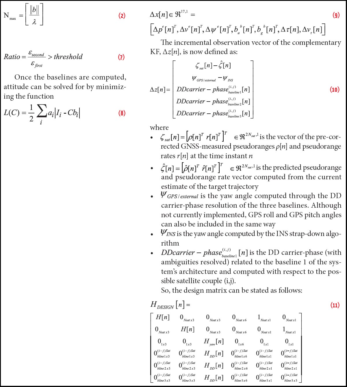
If the baseline length is fixed and known, as in the present case, only a maximum number of integer cycles can fit between antennas. This number is reached when the baseline is rotated parallel to the satellite’s line of sight vector. The maximum number of integers is calculated as the baseline length divided by the carrier wavelength, rounded downwards, thus:
Equation (2) (see inset photo, above right)
The baseline can be rotated 180 degrees with the integer being negative, or can be at right angles with the satellite’s line of sight in such a way that the integer could be zero. In this way, the number of ambiguity candidates comes down to 2Nmax+1. Not all combinations of integers are possible when combining several satellites, but if a brute force algorithm was used, the number of possible integers would be (2Nmax+1)p with p being the number of ambiguities.
Attitude information from the inertial sensors combined with its predicted accuracy can be used to reduce the three-dimensional search space containing the remote antennas. Figure 6 shows an example of this.
The guessed baselines are generated in such a way that they cover the whole attitude range, while they are equally spaced. The angular step θ between two baselines is the angle that gives, at most, a whole wavelength of phase difference from one baseline to the other for any given satellite direction. To compute the individual baselines a least squares approach has been chosen due to its reliability and the reduced number of ambiguity candidates expected. Equation (3) represents the least squares problem:
Hb = ∇ΔΦ – λ∇ΔN – ε(Δφ) (3)
where H consists of double-differenced LOS vectors, b is the baseline, ∇ΔΦ represents the carrier phase double differences, and ε(Δφ) is the residual double difference (DD) noise.
To obtain the coordinates of the individual baseline, the over-determined equation system must be solved in the following way:
b = (HTH)-1HT(∇Δφ – λ∇ΔN) (4)
At this point a sequence of tests must be undertaken to reduce the number of candidates to one for each baseline. First, a test of residuals is executed. The phase residuals are defined as the difference between the carrier phase difference measured by two antennas/receivers forming a baseline and the computed phase difference derived from the baseline vector estimation and satellite line-of-sight vectors. In formulas, the phase residuals can be defined as:
V = —HB + ∇ΔΦ + λ∇ΔN (5)
where V is the vector containing the phase residuals, H consists of double-differenced line-of-sight vectors, b is the baseline, and ∇ΔΦ represents the carrier phase double differences.
Errors in double-difference carrier phase observations from a multi-antenna system mainly arise from multipath effects and the receiver noise. Under favorable conditions when multipath is low, the double-differenced carrier phase residuals generally exhibit a Chi-square distribution (sum of squares of independent random observations having a standard Gaussian distribution). Based on this observation, the quantification of the agreement between measured and computed observations can be made using the quadratic form of residuals:
VTC-1obsV ≤ x2ƒ,1-α (6)
Where x2ƒ,1-α is the Chi-square percentile corresponding to the degrees of freedom f (equal to the number of satellites minus four) and the confidence level 1 – α. Cobs is the covariance matrix of the observations. When the ambiguity candidate fails a test, the tested solution is discarded and removed from the list of candidates.
At this point the baseline geometry test is invoked. A parameter K, selected by the designer, represents the array size of the surviving candidates (i.e., the ones that provide the best results after the geometry test is executed) with respect to the whole search space.
In real conditions, K best solutions for each baseline should be considered to avoid discarding the correct solutions, i.e., retaining only the K solutions of each list of baseline candidates {b1(K),b2(K),b3(K)} with smaller baseline length errors obtained in the test of residuals. Then, these K best solutions are combined by means of the baseline geometry test which generates a list of baseline combinations rank-ordered by an associated error, which is obtained as a function of baseline length and known distances between baselines.
The geometry test takes advantage of the knowledge of not only the baseline lengths but also the relative position and orientation of the baselines. As mentioned earlier, the baseline geometry test exploits the fact that the baselines are not actually independent of each other, as their body coordinates are considered fixed and accurately known. The list of baseline-combination candidates is shortened depending on the obtained error value, which keeps the lower-error candidates on top of the list. Finally, the first- and second-best candidates are used to compute an error ratio in order to ensure that the selected solution can be trusted:
Equation (7) (see inset photo, above right, for equations)
Once the baselines are computed, attitude can be solved for by minimizing the function
Equation (8)
where Ii is the actual i baseline coordinates in the body frame and bi represents the corresponding vector coordinates in the local frame. The ai terms are weight factors, and c is the unknown rotation matrix, which transforms vector coordinates from the local to the body frame. The c matrix that minimizes L(C) can be found using Davenport’s q-method.
Batch Solution
The batch solution is based on the accumulated phase residuals test, which calls for storing the phase residuals that belong to the more likely solutions from several epochs. This test is accomplished after a configurable amount of seconds of processing and storing of data. This accumulation phase is required to observe GNSS signals within a different geometric environment in an attempt to reduce the influence of multipath.
In the following example, the angular search space has been defined as a ±30-degree search for roll and pitch (whose initial values are provided by the MEMS INS) and a full (0–360-degree) search for the yaw angle. In these conditions, the latter angle is completely unknown for a low-cost IMU. The angular steps chosen are 10, 10, and 7 degrees for baselines 1, 2, and 3, respectively. The number of possible baseline solutions is reduced after residuals and baseline length tests, as detailed in Table 1.
After completion of the geometry test, the candidate that shows the lowest error is selected as the “correct” solution and the algorithm can switch into “On-the- Fly” mode.
On-the-Fly Solution & Attitude Results
The algorithm for on-the-fly (OTF) ambiguity resolution is intended for use under dynamic conditions and is initiated with fixed ambiguities obtained from the “batch algorithm.” Its goal is to determine the correct set of ambiguities in the shortest period of time and with a minimum of computations, using single-epoch phase measurements.
Figure 7 shows an example of the effect of solved ambiguities for a static data collection for each baseline. In particular, it shows roll, pitch, and yaw angles computed from solved baseline vectors during a static data collection and by means of the batch solution, accumulating residuals during 10 epochs and using six satellites for the computation (so that five ambiguities are obtained: N1, N2, N3, N4, N5). The computed solution is compared with the one obtained from a GNSS reference receiver.
From Figure 7 we can appreciate how our solution in the attitude estimation is quite good, in particular for the heading angle, and differs by only a few degrees for the pitch and roll angles with respect to the reference solution.
On the other hand, Figure 7 shows the roll, pitch, and yaw angles computed from solved baseline vectors, during a static data collection and by means of the OTF solution, using again six satellites and one epoch. As expected, we can see that the OTF solution generates a more noisy solution compared with the results obtained with the batch solution. The attitude data computed through the multi-GNSS antenna platform are then integrated with the INS according to a tightly coupled technique. Details will be explained in the next section.
Navigation Solution Determination
Figure 8 reports the complete block diagram of the proposed navigation system, hosted in the PU. Even if only three GPS receivers are in principle sufficient to have attitude estimation, our choice to use four GNSS devices is made to provide additional redundancy and robustness against partial GPS outage or physical failure of one of the receivers. Double difference measurements, ephemeris, and estimated attitude are fed into the Tightly-Coupled Algorithm at a rate equal to 1 Hz.
The selected low-cost IMU provides three accelerometers and three gyro measurements at a nominal rate of 100 Hz. They are low-pass filtered to mitigate the mechanical vibrations of the UAV, then are used to compute the INS navigation solution according to strapdown mechanization equations described in the article by D. H. Titterton and J. L. Weston cited in Additional Resources.
An efficient real-time implementation of the strapdown inertial navigation algorithm requires the splitting of the computing processes into low- and high-speed segments. The low-speed calculations are designed to take into account low-frequency, large-amplitude body motions arising from vehicle maneuvers. These are used to determine attitude, velocity, and position, whilst the high-speed section involves a relatively simple algorithm designed to keep track of the high-frequency, low-amplitude motions of the vehicle (i.e., coning and sculling computations). See the articles by P. G. Savage in Additional Resources for more details. We have chosen a computation rate for the high-speed segment equal to 100 hertz while the low-speed portion has a rate that can range from 10 to 20 hertz.
The INS solution is blended with the GPS information in an extended Kalman filter (EKF) according to a tightly-coupled method. This filter estimates the navigation solution and the INS errors by using the following parameters as input:
- ranges, attitude, and Doppler outputs computed by the INS device
- Doppler frequency estimated by the GPS base receiver
- satellites’ position and velocity
- double-difference carrier-phase measurements
- estimated attitude from the four GNSS receivers.
The EKF incorporates a 17-state error model that includes position error, velocity error, and attitude error, accelerometer bias, gyroscope bias, clock bias, and clock drift errors, represented as follows:
Equation (9)
Equation (10)
Equation (11)
where:
- H[n] is the Jacobian matrix of the non-linear relationship between the user position and clock and the Nsat pseudoranges ρ1, …, ρNsat. A detailed explanation of H[n] can be found in the Ph.D. thesis by M. Petovello (Additional Resources).
- Hyaw[n] is the measurement design matrix for external heading measurements and can thus be written as given in G. Falco et alia 2013;.
- HDD[n] is the design matrix related to the DD carrier-phase measurement for each baseline, which depends on H[n] and the lever-arm effect. (For a complete formulation, see the article by Y. Yang et alia in Additional Resources).
Observing the expression of H[n], it appears that the DD phase measurements are used to improve the attitude resolution only, not the position accuracy. This is by no means a conceptual limitation, and DD measurements could be similarly added as observations to the current tightly coupled position solution algorithm.
Nevertheless, the main innovation of the new tight-coupling algorithm implemented in our navigation solution is in the use of the DD measurements that are given as input to improve the estimation of the attitude.
Field Tests Results
Our algorithm design took computational complexity into consideration to allow real-time operation in a low-cost, low-power microcontroller. The code has been implemented in C language and is able to run in real time with room for further optimization. It also permits the option of running additional firmware on top of the navigation core, such as a possible integration of control algorithms in the same platform. More details about the firmware design can be found in G. Falco et alia 2014.
We first tested and validated the hardware and software of the developed navigation system on a car and then mounted on board the target UAV. We used two antenna arrays for the land applications two antenna arrays: The first consists of four low-cost GNSS antennas with a relative distance of 50 centimeters, while the second set is formed by professional-grade antennas with stable phase centers and connected to a professional reference receiver. Figure 9 shows the test equipment and the various settings of the GNSS antennas.
Attitude accuracy tests were conducted first in an open-sky situation, then in a challenging urban scenario. Hereafter, we show the results obtained during a drive in downtown Santander, Spain, the whole trace of which is shown in Figure 10. Narrow streets, boulevards, and the presence of high buildings characterize that urban environment, which affected the correct reception of the satellite signals. Moreover, in such a scenario, the DD carrier phase resolution becomes very difficult to achieve, and often attitude must be estimated by using only the IMU information.
Figure 11 depicts the three Euler angles for yaw, pitch, and roll during the test drive. As reflected in the figure, we can only compare the two attitude estimations at a limited number of points because the receiver often experienced time instants where the three Euler angles were not available. In the part of the trajectory where we can measure such angles, we can observe the error in the INS output of pitch and roll with mean errors of 0.5 and 0.8 degrees, respectively. In comparison, the yaw has a mean error that is slightly bigger the one degree.
After having validated the performance of the system on a land vehicle, we further tested it on board the target UAV. The selected end-user application is a four-rotor rotary wing UAV named Anteos (See Figure 12).
The integration within the UAV required three different integration activities board electrical/mechanical, GNSS antennas mechanical, and software integration.
The mechanical integration of the navigation system processor required the board to be free of most of the vibration that a UAV can generate. For this reason, the board was mounted on the payload docking bay of the UAV. The board is aligned with the UAV INS (namely, an attitude/heading reference system, or AHRS) to obtain directly comparable measurements.
The electrical integration consisted of providing the main batteries voltage to a switching power supply.
The integration of the GNSS antenna required a specific carbon fiber structure prototype to be mounted on top of the UAV, allowing the required 50-centimeter baseline between the antennas. Special care was taken to decrease vibration and the flexion of the structure as much as possible during UAV flights. Moreover compared to other low cost antennas, the chosen unit presents an excellent trade-off between minimization of phase center variation and antenna compactness.
On the UAV side, a serial line has been dedicated to communication with the platform. The purpose of this communication is to gather real time measurements from the navigation system and incorporate them on the UAV real-time telemetry daemon, a portion of the UAV control code dedicated to logging telemetries both for instantaneous use within the UAV control law, and for the logging and post-processing of the mission data.
The flight tests compared the measures taken from the new navigation platform and the on-board INS alone, allowing a real-time comparison of the position/attitude solutions taken from the two independent units. As an example, in Figure 13 the latitude and longitude for both units have been converted in the planar displacement with respect to a common point in order to compare the results in terms of meters. The depicted test was taken from motors power on (i.e., around 40 seconds on ground with UAV motors on) and then about 200 seconds of flight.
In Figure 14 we have plotted the attitude solution obtained with our navigation system compared with the reference one.
The integration showed the capability of the system components to be easily combined and to provide accurate measurements on a demanding platform such as a rotary-wing UAV (no preferred directions, no clamping on ground, side movements, strong electromagnetic fields induced by the four electric motors, vibrations, high dynamics). Once the UAV is in flight the general trend of the measurements follows those of the UAV’s INS, even though at some points the reported attitude differs by some degrees from that of the UAV, which would lead the attitude controller onboard the UAV to overreact.
Conclusions
We designed a sophisticated real-time navigation solution that exploits information coming from multiple GPS receivers and a low-cost MEMS IMU. We were able to estimate the attitude of a UAV platform by forming double-difference carrier-phase measurements to feed a tightly coupled GPS/INS integration architecture. In this way, we demonstrated the technical feasibility of an accurate, low-cost navigation system using non-dedicated hardware and its potential application for UAV navigation.
Acknowledgment
The presented results have been achieved within the LOGAM project which has been funded by the European Union’s Seventh Framework Programme (FP7/2007-2013) under grant agreement #277663.
Additional Resources
[1] Acorde Technologies, S.A., website
[2] Aermatica SPA, website
[3] Baroni, L., and H. Koiti, “Analysis of Attitude Determination Methods Using GPS Carrier Phase Measurements,” in Mathematical Problems in Engineering, Vol. 2012, Hindawi Publishing Corporation, Article ID 596396, p. 10, doi:10.1155/2012/596396, 2012
[4] Falco, G., and M. Campo-Cossío Gutiérrez, E. López Serna, F. Zacchello, and S. Bories, “Low-cost Real-time Tightly-coupled GNSS/INS Navigation System Based on Carrier Phase Double Differences for UAV Applications,” Proceedings of the 27th International Technical Meeting of the Satellite Division of The Institute of Navigation (ION GNSS+2014), Tampa, Florida USA, pp:841-857, doi: 10.13140/2.1.4638.4642, 2014
[5] Falco, G., and M-C. Cossio and A.Puras, “MULTIGNSS Receivers/IMU System Aimed at the Design of a Heading-Constrained Tightly-Coupled Algorithm,” Proceedings of the International Conference on Localization and GNSS (ICL-GNSS 2013), Turin, Italy, doi: 10.1109/ICL-GNSS.2013.6577263, 2013
[6] Mehut. Y., and C. Delaveaud and S. Bories, “Low-Cost GNSS Antennas Phase Center Variations Characterization for UAV Attitude Determination Application,” Proceedings of AMTA 2013 35th Symposium, Colombus, Ohio USA, October 7–10, 2013
[7] Petovello, M., Real-time Integration of a Tactical-Grade IMU and GPS for High-Accuracy Positioning and Navigation, Ph.D. Thesis, Department of Geomatics Engineering, University of Calgary, Canada, UCGE Report No. 20173
[8] Savage, P. G., “Strapdown Inertial Navigation Integration Algorithm Design Part 1: Attitude Algorithms,” Journal of Guidance, Control and Dynamics, Volume: 21, Number: 1, pp. 19 – 28, 1998
[9] Savage, P. G., “Strapdown Inertial Navigation Integration Algorithm Design Part 2: Velocity and Position Algorithms,” Journal of Guidance, Control and Dynamics, Volume: 21, Number: 2, pp. 208- 221, 1998
[10] Strang, G., and K. Borre, Linear Algebra, Geodesy and GPS, Willesley-Cambridge Press, ISBN-10: 0961408863
[11] Titterton, D. H., and J. L. Weston, Strapdown Inertial Navigation Technology, 2nd ed., Paul Zarchan, Editor, ISBN:1-56347-693-, 1997
[12] Wei, Z., “Positioning with NAVSTAR, the Global Positioning System,” Report No. 370, Department of Geodetic Science and Surveying, The Ohio State University, Columbus, Ohio USA, 1986
[13] Yang, Y., and A. Farrel, “Two Antennas GPSAided INS for Attitude Determination,” IEEE Transactions On Control Systems Technology, Volume: 11, Number: 6, pp. 905-918, doi: 10.1109/ TCST.2003.815545, 2003