A GNSS single-antenna system can be compared to a single-pixel camera. Electromagnetic waves traveling 20,000 kilometers from every overhead direction can reach us. Yet once at the antenna, this diverse set of information is collapsed into a single magnitude and phase value, then sent off to the receiver so that value can be extracted.
A GNSS single-antenna system can be compared to a single-pixel camera. Electromagnetic waves traveling 20,000 kilometers from every overhead direction can reach us. Yet once at the antenna, this diverse set of information is collapsed into a single magnitude and phase value, then sent off to the receiver so that value can be extracted.
Antennas can redeem themselves by adding some features, but generally at the cost of greatly increased complexity. Most antenna systems that provide additional functionality rely on multiple antenna elements and multiple analog-to-digital converters (ADCs).
This extra hardware and processing is often used for the simultaneous reception of a single-incident waveform at multiple phase fronts, as is done for example, in a multi-antenna array system. The simultaneously received signals are phase coherent components of the incident waveform: similar in magnitude but shifted in phase. Functionality, such as beam/null steering, can be accomplished by phase shifting and then combining the signals to obtain constructive and destructive interference.
In fact, our proposed single-antenna design is very similar to these multi-antenna systems. However, instead of introducing dedicated antenna infrastructure, we reuse the (already very necessary) body of the airplane fuselage. When our antenna is mounted on a large ground plane, it can resolve two phase coherent components from a single incident waveform. A simple circuit inside the antenna can then introduce the appropriate phase shift to one of the signals and combine the two signals to obtain constructive and destructive interference.
This antenna has three primary modes of operation for this antenna. During the “normal” mode, the antenna performs comparably to standard GPS antennas. During the “anti-jam” mode, null steering toward the optimal azimuthal direction will generally provide greater than 10 decibels of signal suppression. Finally, during the “spoof detection” mode, signals originating from a spoofed source will display a characteristic C/N0 pattern recognizable using a standard GPS receiver’s reporting framework.
Our dynamic antenna requires no additional signal processing at the receiver, no additional cable runs to the antenna, and it fits into the form factor of a standard GPS antenna. This article will describe the underlying theory, design features, and performance results of the antenna in two field trials.
Building Blocks
Direct signals from GPS/GNSS satellites are right-hand circularly polarized (RHCP) and arrive in the upper hemisphere of a standard receive antenna. Thus, GPS/GNSS receive antennas are designed for sensitivity to RHCP signals in the upper hemisphere. However, in practice, all antennas have some sensitivity to left-hand circularly polarized (LHCP) signals. The total sensitivity of the antenna is sum of the RHCP and LHCP sensitivities.
A performance metric measuring the antenna’s ability to distinguish the RHCP energy from the total energy it receives is called cross-polarization discrimination (XPD), and is defined in decibel units as:
XPD (θ, ϕ) = GRHCP (θ, ϕ) – GLHCP (θ, ϕ) (1)
for each potential signal direction of arrival, or DoA(θ, ϕ), in spherical coordinates where θ represents elevation angle and ϕ represents azimuth angle. G represents the RHCP or LHCP antenna gain in that given direction. Note that we refer to gain and sensitivity interchangeably due the reciprocal nature of a passive antenna.
GPS antennas are designed to maximize XPD in the upper hemisphere, because the presence of any upper hemispheric LHCP sensitivity proportionately reduces the antenna’s sensitivity to the satellite’s RHCP signals. At this time we will focus on only the RHCP gain of the antenna, but the LHCP gain will become significant shortly.
The RHCP gain achieved by our antenna is shown in Figure 1, with an example of the constructive (on the right) and destructive (on the left) interference radiation patterns. The traces in these plots show two perpendicular 2-D cuts of a single 3-D radiation gain pattern. Specifically, the blue solid traces represent the static baseline 3-D radiation pattern and the green dashed traces represent the dynamic 3-D radiation pattern that arises when a null has been steered along the 90-degree azimuthal plane. Both patterns were derived from the same simulated data of a standard form-factor GPS antenna on an 800-millimeter diameter by 1,200-millimeter length cylindrical ground plane.
When comparing the baseline RHCP radiation pattern to our “combo’’ RHCP radiation pattern, we can see significant nulls (greater than 10 decibels) and modest “beams” (approximately 3 decibels) appearing in the lower hemisphere of the plots for these two azimuthal cuts. One can imagine that the combo pattern arises when the baseline pattern is squeezed along one 2-D plane, and thus slight bulging appears along the perpendicular plane.
The significance of these two patterns is:
1. The dynamic component of the combo radiation patterns is largely in the lower hemisphere, while the upper hemisphere remains unperturbed.
2. The nulls are quite deep and over a relatively wide range of elevation angles, (comparable to null depths that could be expected from much larger multi-antenna array systems).
The term “combo RHCP” refers to the fact that the radiation pattern is still predominately sensitive to RHCP energy (particularly in the upper hemisphere), despite the combination of signals that takes place in our circuit. As can also be seen in the figures, due to the symmetry present in our single-antenna element, when a null is steered to the 90-degree azimuthal plane, nulls will arise in both the +90 and the –90 degree azimuthal angles. It is important to point out that these two plots — a null radiation pattern and a beam radiation pattern — are the building blocks for all the applications we later introduce.
Theoretical Background
We all know that electromagnetic waves can propagate through both free space, such as the space between the GPS satellites and our antenna, and along conductive structures, such as the coaxial cables that deliver the electromagnetic wave from the antenna to our receivers. However, less obvious is that certain mediums and geometries only support certain types of electromagnetic fields. The waves that travel from the satellites to our antenna take the form of transverse electromagnetic plane waves.
In the case of GNSS, the electromagnetic plane waves are RHCP. An RHCP wave can be decomposed into two orthogonal electric field components (which we can call an x-axis field and a y-axis field for some arbitrary coordinate system in the plane parallel to the plane wave). These two field components are not only orthogonal in space, but also in time, with the x-axis field lagging the y-axis field by 90 degrees.
When an RHCP wave is directly incident upon an RHCP antenna, the two orthogonal electric field components will excite both feeds on the antenna, with a portion of the wave energy lagging by 90 degrees in time. Contrarily, when an RHCP (or any arbitrarily polarized) wave is directly incident upon the conductive ground plane, the electromagnetic wave will induce surface currents along the ground plane.
Despite the considerable losses endured in this transmission mechanism, some of these surface currents will travel along the body of the ground plane until they reach the antenna where they will induce a potential difference between the ground plane and the conductive patch of the antenna. Unlike the RHCP wave incident directly upon the antenna, in this case there will be no 90-degree time shift between any energy that may excite the two feeds of the antenna. In other words, the energy field will be present at both antenna feeds at the same instant, without the time delay characteristic of circularly polarized fields. For this reason, the electric field induced by a surface current is electrically similar to that induced by a vertically polarized (VP) electromagnetic plane wave, and thus we refer to these signals as VP.
One significance of a vertically polarized field in GNSS is that we can be quite confident that it did not originate directly from a GNSS satellite. (Note that some low-elevation GNSS satellite waveforms can appear largely VP to a patch antenna, as will be addressed later). Specifically, for an antenna atop a large cylindrical ground plane (such as an aircraft), any signals that reach the antenna due to the propagation of surface currents will presumably do so because a direct path to the antenna is blocked by the ground plane, and therefore these signals must originate from beneath the horizon of the antenna. Thus, for the coming theoretical conversation, we will assume VP fields are due to waveforms that only originate from elevation angles below the horizon of the antenna.
Another significance of a VP signal is that it can be further decomposed into an RHCP signal and a LHCP signal, with both signals having equal magnitude and phase coherency. We will see later that a standard GPS antenna can easily provide the LHCP signal in addition to the RHCP one. We can also see that a VP signal has an XPD ratio of 0 decibel due to its RHCP and LHCP components having equal magnitude.
So, we have found what we’ve been looking for. We simultaneously have an RHCP and an LHCP signal, which are phase coherent components of the incident waveform: similar in magnitude but shifted in phase. It turns out that the relative phase shift between these two signals is a function of azimuthal angle from which the original waveform originated. In order to achieve a null toward that azimuthal angle, our circuit must introduce an additional phase shift, such that when added to the relative phase shift we obtain a 180-degree phase difference between the RHCP and LHCP signals.
As we developed in prior work (see the paper by E. McMilin et alia listed in the Additional Resources section near the end of this article), our circuit can introduce a relative phase shift ψ in order to steer a null toward ϕ as follows:
Ψ = 2(ϕ − ϕ0) + 90°
where ϕ0 = azimuthal angle of x-axis feed (simply to establish a relative coordinate system), and ϕ = desired azimuthal angle for null.
Although there isn’t room to derive this equation here, it is sufficiently simple that we can describe most of the terms in the equation. The fact that ψ has twice the periodicity of ϕ can be understood from revisiting Figure 1, where we saw that symmetry caused a null to appear simultaneously at both the +90 degree and the -90 degree azimuthal angles. Additionally the fixed term in the equation equal to 90 degrees is there to compensate for the additional 90 degrees introduced by the 90-degree hybrid coupler.
After introducing the required phase shift to the RHCP signal, the final step is simply to combine the shifted versions of the RHCP and LHCP signal to obtain destructive interference. Some concern may arise upon hearing that we are intentionally canceling out part of the received RHCP signal. The next paragraph will address this concern by considering what happens at higher elevation angles.
We have described how the null gets steered in azimuth, but how about elevation? In fact there is no dynamic component that can steer the null in elevation. Rather, the nulls and beams are fixed to the lower hemisphere. Recall this technique works only when the received RHCP and LHCP are similar in magnitude, or have an XPD ratio approaching 0 decibel.
By design, most GPS antennas have XPD ratios exceeding 13 decibels in the majority of the upper hemisphere. Equivalently, the RHCP gain in the upper hemisphere is generally at least 20 times stronger than the LHCP gain. Consequently, the greatest null/beam we would achieve in upper hemisphere is only a five percent reduction/increase in gain (assuming an ideal circuit implementation).
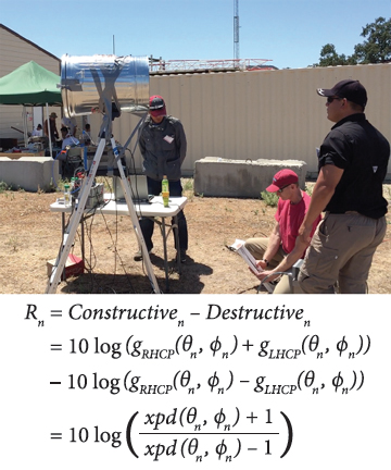
Upon processing in a GPS receiver, an apparent ripple in carrier-to-noise density (C/N0) would arise from periodic combinations of constructive and destructive interference described earlier. The ripple in decibel-hertz (dB-Hz) for the nth satellite can be calculated as:
(For equation, see inset photo, above right)
where (θn, ϕn) are the elevation and azimuth angles of the nth satellite being tracked and the antenna gain, g, and cross polarization ratio, xpd, are shown in lower case to indicate that we are specifying the linear representation of the term, instead of its decibel representation (as is done otherwise in this article).
Note that as the magnitudes of the RHCP and LHCP signals become more similar (or the XPD ratio approaches 0 decibel), the C/N0 ripple approaches infinity. Thus, we could ideally steer an infinitely deep null toward an azimuthal direction in the lower hemisphere where the XPD ratio equals 0 decibel.
Circuit Model
Figure 2 shows a high-level schematic diagram of the system we built. When the switches are in the green state, the block diagram represents a standard GNSS antenna and in this state will serve as the model for the baseline RHCP mode or “normal mode” signals plotted later in this article. When the switches are in the blue state, the diagram is showing the implementation of our anti-jam and spoof detection technique and also serves as the model for the combo RHCP radiation patterns we have already seen.
As indicated in the figure, all the components are housed inside the antenna assembly, with only a single coaxial cable connecting the antenna assembly to the GPS receiver. The only implementation difference between our anti-jam and spoof detection techniques is how the executive function controls the switches and the variable phase shifter, as will be discussed in the next section.
In Figure 2, we can see that the 90-degree hybrid coupler has two output ports, labeled as “RHCP” and “LHCP” and two input ports labeled “x-axis” and “y-axis.” Note that even genuine signals from high-elevation GNSS satellites will deposit a small amount of LHCP energy at port 4. This LHCP energy can derive from many sources, such as atmospheric effects and antenna imperfections. Additionally, GNSS multipath components will have changed from RHCP to LHCP after a single bounce. To mitigate these and other negative effects, the LHCP energy is generally deposited directly into a resistive load, as shown in “normal mode.”
As compared to signal path of the normal mode, in the anti-jam and spoof detection mode two additional components have been added: a variable phase shifter and a Wilkinson power combiner. These two additional components complete the task of phase shifting the RHCP signal component to the ideal ψ value, such that it’s 180 degrees out of phase with the LHCP one, and then combining the two to achieve a null steered in the desired ϕ direction.
Practical Null Steering
Thus far we have discussed a deterministic mapping between an azimuthal angle of interest, ϕ, and the ideal phase shift, ψ. The main purpose of explaining the math behind this mapping is to motivate the necessity of the variable phase shifter. In this section we discuss a more practical mapping between the variable phase shifter and steering of a null in an azimuthal direction, using our anti-jam mechanism as an example.
Although a manually controlled hardware arrangement could be imagined, a more desirable implementation would involve integration with a standard GPS receiver to include a power-minimization algorithm running on the receiver in the digital domain. This algorithm can adapt a DC voltage control signal that is coupled onto the inner conductor of the RF coaxial cable in order to establish an optimal phase shift. The automatic gain control (AGC) could be one low-complexity and backward-compatible mechanism for implementing the power-minimization algorithm.
Full receiver integration would only require a firmware upgrade that links the output of the AGC to the voltage signal that controls the phase shifter in the antenna, with a feedback loop that will settle at the AGC’s default (interference-free) baseline level. The inner conductor of the coaxial cable would also continue to serve in its normal capacity to power the LNAs (and other components) inside the antenna assembly, and thus some simple power-smoothing circuitry would have to be implemented such that the nanosecond duration dips in voltage do not adversely effect the LNAs. As was done in our prototype, a microcontroller would likely reside inside the antenna assembly to control predetermined functionality based on the control voltages received.
Experimental Set-Up
We participated in two field trials where we were able to test our theory, subjecting our prototype to live jamming and spoofed signals while tracking genuine satellites overhead. Both trials were conducted during the Naval Postgraduate School’s Joint Interagency Field Experimentation (JIFX) program on May 12 and August 11, 2015, at Camp Roberts, California, USA.
In the first field trial we ran hardware-in-the-loop tests with traces recorded in a software defined radio (SDR). Most of the anti-jam and spoof-detection functionality was implemented in software. In the second field trial we built a hardware prototype using a commercially available off the shelf hardware and connected it to a triple-frequency GNSS receiver capable of receiver GPS, GLONASS, and satellite-based augmentation system (SBAS) signals. Another difference between the two trials is that in the second one we used an RHCP antenna to transmit the spoofing signals, whereas in the first trial a VP transmit antenna was used. The use of an RHCP transmit antenna was important for validation that an arbitrarily polarized jamming/spoofing signal can be transformed into a VP signal by the large ground plane of an airplane fuselage.
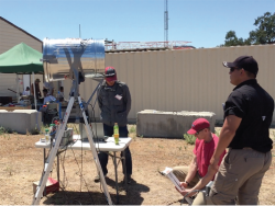
Members from the U.S. Army’s Joint Vulnerability Assessment Branch (JVAB) were on site to support both of our field trials. The top image in Figure 3 shows the GNSS simulator used by JVAB to generate the spoofed GPS signal shown in the bottom image of the figure. This signal was generated in band at a center frequency of 1575.42MHz with –65dBm of power in the first field trial and –75dBm of power in the second field trial. To minimize impact upon other nearby experiments, JVAB spoofed for a position in China, thus generating signals for a largely non-overlapping set of GPS satellites and with different dopplers than the genuine overhead satellites.
In both field trials we used the spoofed signal to serve as both a jamming source and a spoofing source, simultaneously. Thus, the spoofed signals will generally appear at a peak higher C/N0 value than the genuine signals. However, the peak C/N0 value is not relevant to the spoof-detection technique we employ.
Antenna
For these field trials we designed and fabricated a simple GPS patch antenna that we expect to be consistent with existing patch antennas and that meets ARINC 743 form-factor constraints. The antenna, shown in Figure 4, is a 40×40-millimeter substrate with a 30×30-millimeter copper patch on top and is very similar to the antenna that we simulated earlier in this article. The substrate, at 1.28-millimeter thick, is a single layer of Rogers RO3010 material that has a dielectric constant of 10.2. This high dielectric constant allows us to create a relatively small form-factor half-wavelength resonant antenna.
The patch antenna has two perpendicular coaxial feeds. We select a coordinate system such that we call one of the feeds the x-axis feed and the other the y-axis feed, as shown in Figure 4.
This antenna was designed to be mounted on a large conductive body, such as the fuselage of an airplane. In the case of this field trial the antenna was mounted on a metal trash can that served to emulate the cross-section of an airplane fuselage. Specifically, the antenna was affixed to a standard 31-gallon galvanized steel trash can with a 533-millimeter (21-inch) diameter and a 685-millimeter (27-inch) length, again similar to the ground plane we simulated earlier in this article.
Although we hope to replace the trash can with an actual aircraft one day, for the time being any relatively large ground plane will serve to validate our technique. Furthermore, we expect improved results as the ground plane increases in size as we have shown in our prior work. Before we began the measurement, we affixed the antenna plus trash can assembly atop a small ladder, just less than two meters high, as can be seen in the accompanying photo (see inset photo, above right).
Field Trial #1
Figure 5 presents a block diagram version of the hardware setup for the first field trial. In this trial, coaxial cables connect the two ports of the patch antenna into a two-port SDR. Signals on these two parallel paths were sampled at a rate of 5Msps. Both receive channels use the common internal clock; however, we have instead elected to use an external 10-megahertz rubidium oscillator for improved clock stability of less than two picoseconds over a 100-second interval. Finally, the SDR is connected via USB3 cable to a laptop to record the raw I/Q samples that are captured from each stream.
We did not perform any real-time processing on the recorded samples. Thus, during the field measurement we were blind to the performance of the positioning, navigation, and timing (PNT) solution and the degradation that the jamming and/or spoofing may be inflicting upon that solution.
Anti-Jam in Field Trial #1. For the first field trial, we had the benefit of not needing to change states between normal mode and anti-jam mode, but instead we could view the results of both states in parallel. However, because we did not implement any feedback-loop mechanism, we had to theoretically determine the phase shift required for optimal null steering. Given the orientation of our antenna and the direction of the jamming signal, the calculated optimal phase shift is –90 degrees.
In post-processing we used a one-degree step size to sweep a range of phase shift values around our calculated optimal value. We determined qualitatively that a phase shift of –73 degrees produces the optimal results, suggesting an 8.5-degree error in our estimation of our relative azimuth angle. Figure 6 compares the Stanford GPS SDR’s results for the direct “Normal mode” stream (in green) and the “Anti-jam mode” stream (in red), when the variable phase shifter has been set to a value of –73 degrees (and thus steered a null toward the direction of the jamming signal).
The figure includes a sky map with a black dotted line to indicate the direction of the x-axis antenna feed and a purple arrow to show the direction of the jamming signal perpendicular to the direction of the x-axis antenna feed. Note that satellite PRN 17 is almost directly overhead, satellite PRN28 is in the direction of the spoofed signal, satellites PRN 15 and PRN 30 are approximately orthogonal to the direction of the spoofed signal, and satellites PRN 6 and PRN7 are at low elevation angles.
Table 1 shows the test sequence. We can see that the drop in the green normal mode C/N0 is correlated with the increase in the elevation angle of the horn transmitting the jamming signal. When the jamming signal is incident upon the “fuselage” at a lower elevation angle, it must propagate along the ground plane for a longer distance before it reaches the antenna, and thus is further attenuated.
As the jammer increases its elevation angle up to the horizon of the antenna, however, the effective signal strength of the jammer increases despite no change in the transmission power level. Consequently later in the signal recording we are more likely to see a loss of lock on satellite signals. This is particularly the case for the lower-elevation satellites (PRNs 6, 7, and 15), which already had a lower initial normal mode C/N0 prior to the introduction of the jamming signal.
Now, turning to the red anti-jam C/N0 traces, we see jam suppression ranging from about 10 decibels to greater than 20 decibels. Anti-jam performance for the high-elevation satellites (PRNs 13, 17, and 30, but excluding satellite PRN 28) increases to around 10 decibels of jam suppression. Furthermore, jam suppression of the lower-elevation satellites (PRNs 6, 7, and 15) as well as PRN 28 is generally 20 decibels or better, avoiding a loss of lock for several satellites (when compared to the normal mode performance).
By coincidence, the spoofing signals are originating from the same direction as satellite PRN 28 (sky plot in lower right-hand corner of Figure 6); thus, a radiation pattern null has been formed along a line in the azimuthal plane that is parallel to satellite PRN 28. Simultaneously, a slight radiation pattern beam has been formed along the line perpendicular to the direction of the spoofer in the azimuthal plane (indicated by the black dotted line on the sky plot). This dotted line happens to run between satellites PRN 15 and PRN 7. Thus, in satellite PRN 28 we see a slight reduction in anti-jam mode C/N0 as compared to normal mode C/N0 before the jamming signal has begun to degrade the normal mode C/N0 (and we also see more dramatic jam suppression as the effective signal strength of the jammer increases).
Contrarily, in satellites PRNs 15 and 7, we see a slight increase in the anti-jam mode C/N0 as compared to normal mode C/N0 even before the jamming signal has begun. This superior performance of anti-jam mode C/N0 as compared to normal mode C/N0 continues for satellites PRNs 15 and 7 as the effective jamming signal strength increases, because of the compounded effects of the beam steered toward these two satellites and the null steered toward the jammer.
Spoof Detection in Field Trial #1. We assume an evasive and sophisticated spoofer that would attempt to avoid triggering any detectable AGC decrease or C/N0 increase. Thus we are forced to deterministically steer the variable phase shifter through all 360 degrees to provide visibility in every possible direction of attack. The Stanford GPS SDR has a coherent integration time of 20 milliseconds and the C/N0 output rate is 2.5 hertz (or computed every 400 milliseconds). To avoid excessive smoothing of the C/N0, we pause for a 800-millisecond interval every 10 degrees, completing a full 360-degree revolution of phase shifter values every 28.8 seconds.
Figure 7 shows the results of implementing both the spoof-detection process and the normal-mode process in parallel. Recall that the spoofer signal here is the same signal that was previously serving as a jammer. However, this time we have adjusted the Stanford GPS SDR to also track the spoofer signals.
Similarly as before, we see the spoofer signals begin at around 120 seconds. The green normal-mode C/N0 traces report these spoofed signals as “genuine” satellites. However, looking at the red spoof-detection traces, the amplitude of the C/N0 ripple provides a distinction between the genuine and the spoofed signals.
As calculated earlier, the amplitude of the ripple in C/N0 that we see in Figure 7 has an inverse relationship to the XPD. Generally speaking the XPD is higher for high-elevation satellites and lower for low-elevation satellites. For the spoofed signals originating from below the horizon, we expect the XPD to approach a value of 0 decibel, leading to large amplitude swings. As expected, we see a quite low amplitude swing for the higher-elevation satellites (PRNs 17, 13, 28 and 30), a larger amplitude swing for the lower-elevation satellites (PRNs 6, 7, 15), and the largest amplitude swing for the spoofed satellites (PRNs 1, 4, 20, 27, 32).
Note also that each unique satellite has its own swing amplitude and phase offset in the time domain of where the peaks and troughs fall during the 28.8-second cycle. However, all the satellites spoofed from a single location will share the same C/N0 amplitude and time domain offset with one another. Analysis of our second field trial results in the following section will investigate this result and further address the distinction between low-elevation satellites and spoofed signals.
Field Trial #2
Figure 8 identifies the components of the antenna prototype tested in our second field trial. For flexibility, we built the prototype with the components implemented on evaluation boards. All of the components are low in cost and commercially available off the shelf.
The elements in our prototype match those shown in the schematic (Figure 2), with the addition of three additional elements highlighted in dark gray: a signal generator and DC amplifier to control the variable phase shifter, and an Arduino micro-controller to control the switches. These three additional components replace the “Executive function” block seen in Figure 2, and would be further integrated in a commercial realization of the antenna.
We elected to use an analog voltage-controlled variable phase shifter for ease of implementation, but one trade-off in this decision is the two-decibel insertion-loss ripple as a function of phase that is inherent to the component. This insertion-loss ripple is superimposed upon any C/N0 ripple that we had expected from our null/beam steering and may limit the depths of our nulls.
Anti-Jam in Field Trial #2. Figure 9 shows the C/N0 values for 10 satellites signals tracked by the NovAtel during our anti-jam experiment. Because we did not implement an AGC or C/N0 feedback mechanism to steer the variable phase shifter, we instead used the signal generator to slowly ramp through all 360 degrees of phase shift values over an approximately 60-second duration, which serves as the x-axis in our plots. During the entire 60-second duration, the spoofed signal was at an azimuth angle of 180 degrees (parallel to the direction of the x-axis antenna feed) and an elevation angle of 90 degrees (at the horizon of the antenna).
Because the jamming signal was actually a spoofer, we are able to see both the suppression of the spoofed satellites signals in parallel with the recovery of the genuine signals. Specifically, we see that the four spoofed satellites signals (PRN 8, 10, 26, 27) suffer greater than 15 decibels of signal suppression when the optimal phase shift value has been reached.
Approximately 3 decibels of jamming signal suppression is seen from 120 seconds to 140 seconds, and during that interval several genuine satellite signals reestablish lock (PRN 2, 6, 24, 28). All of the genuine satellite signals appear to show improved performance when the jamming effects of the spoofing signal has been suppressed.
Spoof Detection in Field Trial #2. Figure 10 shows the C/N0 values for all 10 satellites signals tracked by the NovAtel for the spoof detection aspect of our experiment. To permit rapid detection while avoiding excessive smoothing of the C/N0 ripple, we set the signal generator to ramp through all 360 degrees of phase shift values in a five-second duration. We then held the spoofing transmit antenna at given elevation angle for a little over 20 seconds before transitioning to another elevation angle.
The x-axis in the Figure 10 plots shows time progression, modulo 20 seconds. During the entire experiment the transmitted spoofed signal originated from an azimuth angle of 180 degrees and elevation angles of 90 degrees (at the horizon of the antenna), 120 degrees (30 degrees below the horizon of the antenna), and 150 degrees (60 degrees below the horizon of the antenna).
Again, as in the first field trial, we see that when the spoofing signal’s effective signal strength is increased as its elevation angle up increases. Because the GNSS receiver was tracking both genuine and spoofed signals, we can compare the characteristic C/N0 behavior of both signal types. First, focusing on the green and red traces (captured when the spoofer was below the horizon of the antenna), we see that signals from the four spoofed satellites (PRN 8, 10, 26, 27) display the expected large C/N0 ripple. This large C/N0 ripple alone could be sufficient to classify these four signals as spoofers.
However, when we focus on the blue trace (captured when the spoofer was at the horizon of the antenna), we don’t see a larger ripple in the spoofed signals, as compared to the genuine signals. This could be because the receiver was partially saturated by the high signal power coming from the spoofed signal and/or because the RHCP signal had not been transformed into a predominately VP signal at the time it reached the antenna. Another causal and/or contributing factor could be that the genuine signals are exhibiting excessive C/N0 ripple in response to the periodic suppression and resumption of the strong spoofing signal.
Regardless of the cause, it could be argued that these spoofed signals might easily be misclassified as genuine signals due to the similarity in the magnitude of the C/N0 amplitude ripples shown by both the genuine and the spoofed C/N0 traces in blue. However, as we mentioned previously, the ripple of the maximum and minimum C/N0 values are a function of the elevation angle of the satellite, and the time offset at which those max/min values appear is a function of the azimuth angle of the satellite. We’d thus expect a unique C/N0 ripple for each satellite in the sky.
To examine this assumption more closely, we ran a simple script on an arbitrarily selected five-second interval of the blue C/N0 traces shown in Figure 10. This script extracted the max/min C/N0 values and the relative phase offset (within the five-second cycle duration) at which those max/min values occurred.
Table 2 shows that the standard deviation in the maximum and minimum C/N0 values for the five genuine satellites is more than 10 times larger than that of the four spoofed satellites. Similarly, the standard deviation of the phase offset for the maximum and minimum C/N0 values for the five genuine satellites is about 50 times larger than that of the four spoofed satellites.
Unlike the previously reported results, this last finding does not depend on the presence of a large ground plane underneath the antenna. Nor does is depend on the spoofed signals originating from below the horizon. Rather, the absence of a unique C/N0 ripple for each satellite indicates that the satellite signals are not originating from unique locations in the sky. This conclusion can be reached regardless of where the spoofed signal may originate.
Acknowledgments
The research conducted for this paper took place at the Stanford University Global Positioning System Research Laboratory with funding from the WAAS program office under FAA Cooperative Agreement 12-G-003. Thank you to Abiud Jimenez, David Rohret, and their colleagues at JVAB for their generous support during our field trials.
Additional Resources
[1] Chen, Y.-H., and J-C. Juang, J. Seo, S. Lo, D. Akos, D. S. De Lorenzo, and P. Enge, “Design and Implementation of Real-Time a Software Radio for Anti-Interference GPS/WAAS Sensors,” Sensors No. 12, pp. 13417-40, 2012
[2] Chen, Y.-H., and S. Lo, D. Akos, D. S. De Lorenzo, P. Enge, “Validation of a Controlled Reception Pattern Antenna (CRPA) Receiver Built From Inexpensive General-purpose Elements During Several Live- jamming Test Campaigns,” Proceedings of the 2013 International Technical Meeting of The Institute of Navigation, San Diego, California, January 2013, pp. 154-163
[3] Konovaltsev, A., and S. Caizzone, M. Cuntz, M. Meurer, “Autonomous Spoofing Detection and Mitigation with a Miniaturized Adaptive Antenna Array,” Proceedings of the 27th International Technical Meeting of The Satellite Division of the Institute of Navigation, Tampa, FL, September 2014, pp. 2853-2861
[4] Kraus, T., and F. Ribbehege and B. Eissfeller, “Use of the Signal Polarization for Anti-jamming and Anti- spoofing with a Single Antenna,” Proceedings of the 27th International Technical Meeting of The Satellite Division of the Institute of Navigation, Tampa, Florida USA, September 2014, pp. 3495-3501
[5] McMilin, E., and D. S. De Lorenzo, D. Akos, S. Caizzone, A. Konovaltsev, T. H. Lee, P. Enge, “GPS Anti-Jam: A Simple Method of Single Antenna Null- Steering for Aerial Applications,” Proceedings of the ION 2015 Pacific PNT Meeting, Honolulu, Hawaii, April 2015, pp. 470-483.
[6] Montgomery, P., and T. E. Humphreys, “A Multi-Antenna Defense: Receiver-Autonomous GPS Spoofing Detection,” Inside GNSS, pp. 40-46, March/April 2009
[7] Rosen, M. W., and M. S. Braasch, “Low-Cost GPS Interference Mitigation Using Single Aperture Cancellation Techniques,” Proceedings of the 1998 National Technical Meeting of The Institute of Navigation, Long Beach, CA, January 1998, pp. 47-58