 Equations
The advent of multiple constellations provides the opportunity to eliminate geometry weakness as a source of satellite-based augmentation system (SBAS) unavailability. GPS users occasionally encounter areas where an insufficient density of satellites exists to support all desired operations. This most often occurs when a primary slot satellite is out of service. However, adding one or more constellations easily compensates for this geometric shortcoming. In fact, we may now experience the opposite problem of having more satellites that can be tracked by a receiver.
The advent of multiple constellations provides the opportunity to eliminate geometry weakness as a source of satellite-based augmentation system (SBAS) unavailability. GPS users occasionally encounter areas where an insufficient density of satellites exists to support all desired operations. This most often occurs when a primary slot satellite is out of service. However, adding one or more constellations easily compensates for this geometric shortcoming. In fact, we may now experience the opposite problem of having more satellites that can be tracked by a receiver.
There are many possible methods for selecting a set of satellites to use for the GPS position solution. Very often, elevation angle is used to rank satellites. A receiver may sort the satellites by their elevation angle and keep k (number of receiver hardware channels) highest ones. While this choice is good from a tracking robustness point of view, it does not lead to the best availability.
Ideally, when choosing from n total satellites in view, the user will be able to find k that produce protection level values that are below the required integrity alert limits. In general, for aviation SBAS users it is desirable to find an algorithm that minimizes the vertical protection level (VPL) and the horizontal protection level (HPL). A brute force search, through all combinations, yields the optimal set for a given k, but may be costly and impractical when there are many possible satellite subsets.
In this article, we examine and compare several methods that are more practical than the “optimal” brute force search. One such method is a “greedy” algorithm that iteratively removes the single least important satellite one at a time until only k satellites remain.
An important consideration is that the optimal set of satellites depends on the specific protection level being minimized. The best sets will be different for SBAS VPL and SBAS HPL. Therefore, we need to define a balance when choosing between deselecting a satellite that least affects the VPL versus deselecting a satellite that least affects the HPL.
Another factor is that the receiver is also capable of reverting to advanced receiver autonomous integrity monitoring (ARAIM) when leaving the SBAS service area – or in the event of an SBAS outage. The optimal satellite sets for ARAIM VPL and HPL differ even further from the SBAS sets; so, we may want to pursue another desirable goal: finding a satellite set that simultaneously allows the SBAS and ARAIM VPLs and HPLs to remain below their respective alert limits. We then use these algorithms to evaluate the decrease in performance relative to the all-in-view protection levels.
We perform this analysis for dual-constellation conditions in order to examine sensitivity to satellite redundancy and geometric strength. Later, different constellation scenarios should be evaluated to determine the robustness of the techniques to initial geometric strength, and total numbers of satellites. This article will address several important questions:
- How quickly the protection levels increase as the number of tracking channels is decreased?
- How should tracking requirements be specified?
- If we specify a minimum number of channels, what is the correct value?
Prior Satellite Selection Algorithms
Specifying a large required number of tracking channels does not automatically assure good performance. Cases will probably always arise in which the receiver cannot track all satellites in view and, as a result, has to choose which ones to track and which to ignore. A poor selection algorithm can lead to poor performance, even when tracking a large number of satellites. Conversely, a relatively small number of satellites may lead to good performance if those satellites are well chosen. This section will describe some commonly understood methods for satellite selection.
Probably the most common satellite-selection method is to use the elevation angle as a discriminator. The receiver may determine elevation angle, given a rough position estimate and the satellite almanac files that describe the approximate satellite orbital locations. The user does not need to track the satellites to estimate their elevation angle for the assumed location. The receiver will determine the elevation angle for every satellite for which it has almanac data. It can then eliminate from consideration signals from all of those satellites whose elevation angle falls below some elevation mask angle (e.g., five degrees as in today’s GPS aviation receivers).
If the receiver has enough channels to track all of the remaining satellites then no further selection is required. However, if more satellites remain than the number of receiver tracking channels, the receiver must choose a set of satellites to track (or equivalently, the complementary set of satellites to exclude).
The “elevation” method sorts the satellites by elevation angle and keeps the k satellites with the largest values. If more satellites are present above the mask angle than the receiver has tracking channels, the lowest elevation satellites are excluded. The lowest elevation satellites typically have the lowest received power and are the most vulnerable to loss due to aircraft banking. However, they are often quite important for good vertical geometry. Removing the lowest satellites can significantly increase the vertical dilution of precision (VDOP) and, in turn, VPL for SBAS and ARAIM.
We should note, however, that the elevation method does not take into account satellite health or weighting factors. Higher elevation satellites may be unmonitored by SBAS or have large variances associated with their corrections. Simply looking at elevation angles discards this additional information.
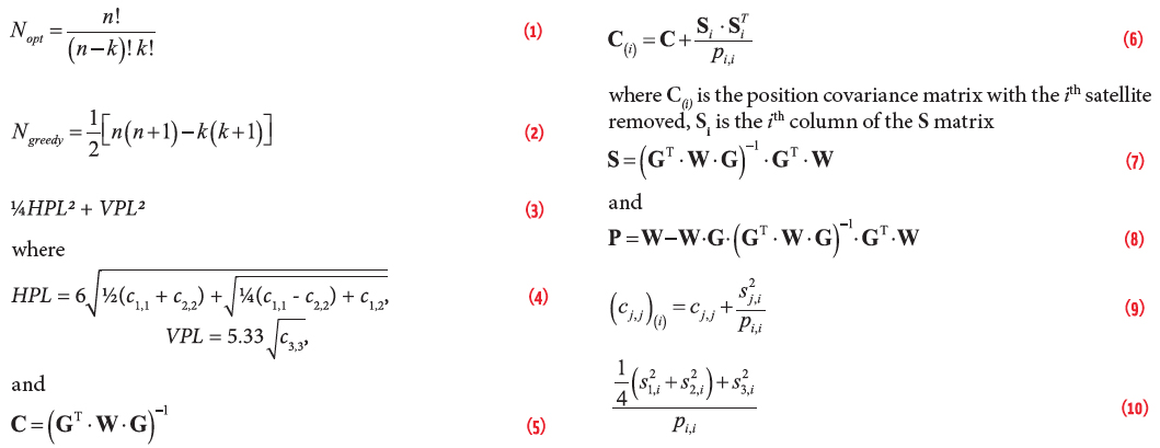
A better method would also make use of the health and weighting information that is broadcast from the SBAS satellites. This information should be used together with the satellite locations. Only satellites designated as healthy by the SBAS should be included in the n satellites to be considered for tracking. An “optimal” brute force method would look at all possible combinations of k out of n satellites to determine the best performance. This method is optimal in terms of returning the best possible outcome, but is distinctly non-optimal in terms of computational cost. If there were n healthy satellites above the mask, a receiver with k channels would have to evaluate Nopt geometries where Nopt is given by
Equation (1) (see inset photo, above right, for all equations)
If n = 30 and k = 24, then Nopt = 593,775 geometries to evaluate. As n becomes larger or k becomes smaller, the number of geometries to evaluate becomes even larger. As we will show later, we can efficiently code subset evaluations without having to compute full matrix inversions for each. However, even with efficient implementations, this approach has significant computational cost. We have used it for a few isolated geometries to compare the optimal result to the results from other methodologies.
The “greedy” method is similar to the optimal in that it evaluates the performance of the subsets. The key difference is that the greedy method removes one satellite at a time and then uses the resulting geometry with the corresponding satellite removed to evaluate the next iteration. For a case with 30 initial satellites, all 30 subsets containing 29 satellites are evaluated. Then the one with the best metric is used for the next step where 29 subsets each containing 28 satellites are evaluated. This continues until only the desired number of satellites remains. The number of subsets to be evaluated by this method, Ngreedy, is given by:
Equation (2)
For n = 30 and k = 24, then Ngreedy = 165 geometries to evaluate. This is certainly more work that the elevation angle method, but far less than the optimal. Ideally, we would like to find a method that has an even smaller computational cost.
A large number of selection algorithms have been developed over time. (See the Additional Resources near the end of this article for some examples.) Many of these seek to minimize the geometrical dilution of precision (GDOP) and do so by maximizing the volume of a polyhedron defined by the satellite locations. However, such methods do not account for the SBAS weights and are therefore not as well suited for our application.
Performance Optimization
In this section we will quantitatively define how we evaluate performance and therefore how we rank one set of satellites as being better than another. The desired property is to maximize availability for SBAS operations. SBAS provides different service levels with different horizontal and vertical alert limits.
If the receiver knows the vertical alert limit VAL and the horizontal alert limit (HAL), it could use a cost function designed to try to keep the VPL and the HPL below these thresholds. Such cost functions would be small while the protection levels are below their respective alert limits but would dramatically increase as the protection level approaches or exceeds these thresholds. However, some classes of SBAS receiver merely output position estimates and protection levels. They do not know which service levels or alert limits are being targeted. Such receivers do not know how much margin they have against the alert limit thresholds.
In the more demanding SBAS services, the VAL is smaller than the HAL. Also, the user almost always has a larger VPL than HPL. Therefore, it is typically much more important to minimize the VPL than it is to keep the HPL small. However, one should take both into account and try to prevent either one from exceeding their respective alert limits. We have therefore chosen to use the following cost function for ranking geometries:
Equation (3)
where
Equation (4)
and
Equation (5)
is the position estimate covariance matrix in the East-North-Up (ENU) frame, G is the geometry matrix (also in the ENU frame), and W is the weighting matrix.
This cost function represents a trade-off between the vertical horizontal protection levels. The factor of ¼ multiplying the square of the HPL shifts priority to minimizing the VPL over minimizing the HPL. This factor is arbitrary and could easily be adjusted to shift the balance in one direction or the other.
Indeed, the cost function itself was subjectively chosen. It was chosen in large part due to its simplicity. We had initially optimized only the VPL but found that sometimes satellite sets were chosen that had large HPL values. We found that by including the horizontal terms as in (3) we prevented large growth in the HPL. There are likely other cost functions that would lead to superior availability, however we believe that (3) is reasonable first choice.
Measurement Downdate Method
Because we are trying to optimize elements of the covariance matrix, we return to the approach of the greedy algorithm. It is trying to identify the subset with the smallest value for (3). Rather than performing n separate matrix inversions to find the n subset versions of C, we can obtain them through
Equation (6)
where C(i) is the position covariance matrix with the ith satellite removed, Si is the ith column of the S matrix
Equation (7)
and
Equation (8)
Thus, starting from a single matrix inversion to obtain the all-in-view position estimate covariance matrix C, we can then find all the subset position estimate covariance matrices using much less computationally costly matrix multiplications rather than inversions.
While this downdate method points to a more efficient means to implement the greedy algorithm, we can see that it also points the way to an even more efficient algorithm. From (6) we can see that
Equation (9)
The last term in (9) represents the increase in the covariance matrix, along the jth user position axis, when removing the ith satellite. The smaller this term is, the less impact it has in increasing the corresponding covariance term. Therefore, if we calculate
Equation (10)
and find the minimum value over all satellites, i, we will approach the cost function of (3).
Most often we will have identified the satellite that the greedy algorithm would choose to exclude at the first step. However, rather than following the greedy algorithm and calculating the covariance matrices for sub-subsets, we can simply sort the values in (10) from the all-in-view calculation and retain the satellites corresponding to the k largest values.
We will call this the “downdate” method. We can see that it is much more efficient than the greedy method. As with the elevation angle method, we determine a set of values once for the all-in-view solution and then use the satellites with the k largest values.
In the elevation method, the retained satellite elevation angles are maximized. In the downdate method, the retained satellite values given by (10) are maximized. Although it requires more effort to determine the downdate values than it does to determine the elevation angles, the downdate method is still very efficient compared to other alternatives.
A similar method was recently proposed for GBAS by Gerbeth et alia (Additional Resources), that uses s3,i to sort satellites. Although s3,i correlates well with VPL, the authors had to add further logic to ensure the minimum VPL was found. For SBAS, s23,i/pi,i is proportional to ΔVPL2, so excluding the satellite with the minimum value directly corresponds to finding the one-out subset with the smallest VPL. In the next sections we will compare the ability of the various selection routines to optimize performance.
Simulation Setup
We used our Matlab algorithm availability simulation tool (MAAST) to create simulated geometries and weights. In order to test the algorithms’ performance against a large number of potential satellites in view, we used a GPS almanac with 31 satellites (as of May 6, 2016), a Galileo almanac with 30 satellites, and the three active wide-area augmentation system (WAAS) geostationary satellites. We simulated both the cur-rent single-frequency (SF) integrity algorithm performance and future dual-frequency (DF) algorithm performance.
We evaluated performance for users spaced on a two-degree by two-degree grid and used 300 evenly spaced time steps over one sidereal day. User positions were constrained to be in a lat/lon box between 15 degrees North and 75 degrees North, and between 175 degrees West and 50 degrees West. This set up was expected to create many different user scenarios, including ones where many satellites were in view, but with very different weights.
The weights in particular are subject to variability. It is uncertain what values will be obtained for the weighting terms by the various SBAS providers, especially in a future DF environment. Thus, the absolute values of the protection levels are subject to change, however, we believe that the relative percentage change due to removing satellites should be representative.
The SF simulation created 158,788 valid position estimates with 23,768 of them having more than 24 usable satellites in view. The DF simulation created 188,200 valid position estimates, with 26,709 having more than 24 usable satellites.
Figure 1 shows histograms for the relative numbers in view for each case. The maximum number in view for this constellation configuration was 31 satellites.
The different simulations created a wide variety of user scenarios featuring different weighting and geometry conditions. We then applied the elevation, greedy, and downdate methods to simulate receivers that had differing values for the maximum number of satellites that could be tracked.
Example Geometry
Figure 2 shows a skyplot for an example geometry corresponding to the dual-frequency simulation and for a user with 31 satellites in view. The numbers in the circles correspond to the PRN/SBAS slot numbers where values from 1 to 32 correspond to GPS, 75 to 111 to Galileo, and 120–158 to SBAS geostationary Earth orbit satellites (GEOs). The coloring indicates the sigma values used to create the weighting matrix.
The SBAS GEOs, as is typical, have much higher sigmas, and therefore, much lower weighting.
Figure 3 shows which satellites are excluded by the elevation, greedy, or downdate method assuming a maximum of 24 satellites can be tracked. Satellites excluded by the elevation method are indicated by the blue pie wedges at the top of the numbered circles identifying the PRNs and location of the spacecraft. Satellites excluded by the greedy method are indicated by the cyan pie wedges at the bottom left of the numbered circles, and those excluded by the downdate method are indicated by the yellow pie wedges at the bottom right of the circles.
Note that the greedy and downdate methods show much better agreement between themselves than with the elevation method. Both greedy and downdate methods agree that PRNs 12 and 92 are the least important satellites. They also both exclude 11, 93, 94, and 104, but not in the same order. Greedy also excludes 103 while downdate also removes 22. Both see relatively small increases in the VPL (three centimeters for greedy and two centimeters for downdate) and somewhat larger increases in HPL (70 centimeters for greedy and 98 centimeters for downdate). Both increases are much smaller than the increases seen by the elevation angle method (3.48 m in VPL and 1.23 m in HPL).
Table 1 shows the HPLs and VPLs for four methods and for the maximum number of channels ranging from 31 down to 20. We also evaluated the optimal brute force method for this table.
The downdate, greedy, and optimal methods are all comparable, even when removing 11 out of 31 satellites. This is particularly impressive because the downdate method only calculates the S and P matrices one time, for the full all-in-view solution. These matrices are not reevaluated after each satellite removal, as is the case for the greedy and optimal methods.
Although these methods may not completely agree on the order in which to remove satellites, we find little difference in performance. They are choosing between roughly equally important satellites; so, the exact ranking is not critical. Contrast this to the elevation method, which is clearly removing satellites that otherwise keep the VPL small.
Which method truly performs better is debatable as it is not obvious how much more important minimizing VPL over HPL is in this case. The last three methods all achieve VPLs below 10 meters and HPLs below 6 meters.
Table 2 shows the order in which satellites are removed when excluding satellites by each method. When the number of channels is reduced by one, a single satellite is excluded from the prior set for the elevation, downdate, and greedy methods. This satellite will not be used for any cases with an even smaller number of channels.
The optimal method, however, completely reevaluates each possible set of satellites. Thus, sometimes satellites that were excluded for a particular number of channels are not excluded for a smaller number of channels. For example, the difference between the satellite set for the optimal method when going from 26 to 25 channels is to reintroduce PRN 11 and remove PRNs 22 and 103.
In the following section we look at statistical performance for the full set of users and time steps.
Simulation Results
Instantaneous availability is determined by whether the VPL and HPL are below their respective alert limits. The example geometry has an all-in-view VPL of 8.88 meters and HPL of 4.34 meters. These are well below the LPV-200 alert limits (VAL = 35 meters and HAL = 40 meters). They are even below the CAT-I autoland alert limits (VAL = 10 meters and HAL = 40 meters).
We could significantly increase the HPL without crossing its threshold; however, the VPL has substantially less margin. This is what motivated the factor of four dividing the horizontal terms in our cost functions. Note that in the example geometry, the elevation angle method does not support CAT-I autoland with fewer than 27 channels, while the other methods support this mode down to at least 20 channels.
Remember that the broadcast sigma values are subject to change, as they depend on future dual-frequency algorithms. If the sigmas were made three times larger, the VPLs and HPLs would also all become three times larger. In that case, the all-in-view solution would still support LPV-200 (but not CAT-I autoland). In such a scenario, the elevation angle method would not support LPV-200 with fewer than 25 channels. The other methods would support it down to at least 20 channels.
Figure 4 shows the maximum observed percentage increase in the protection levels observed for the single-frequency simulation. These values decrease as the number of channels increases.
The elevation method has significantly larger values for the VPL, ranging from a ~5 percent increase at 30 channels, to more than a 100 percent increase for 20 channels. At 24 channels, there was nearly a 50 percent increase.
The downdate and greedy methods show dramatically smaller increases in VPL. They range from less than a 0.2 percent increase at 30 channels to less than 9 percent for 20 channels. These methods saw a ~2 percent maximum increase at 24 channels.
The HPL increases for the three methods are much more similar, but the greedy method has the best performance. For 24 channels, the elevation and downdate methods see up to ~30 percent increase, while the greedy method sees up to ~20 percent. A similar set of curves was obtained for the dual frequency simulation.
Availability is typically specified as an average, which over time requires more than 99 percent of all geometries at a single location to be instantaneously available. We can calculate the effect that having a limited number of channels has on observed availability, but it is harder to generalize the results. They will depend greatly on the assumed constellations and weights. They also will be very dependent on alert limits for the desired operation.
Figure 4 shows the largest observed protection level increases. If such large increases are only rarely observed, they may have little effect on average availability. However, if we evaluate constellations with an even greater number of satellites, the large increases in protection levels will be more common and will have a larger impact on average availability.
Table 3 shows the percent decrease in CAT-I autoland coverage area for the dual-frequency simulation. The coverage region is the area in which a specified availability is met. We determined the coverage region for the all-in-view case corresponding to availabilities, ranging from 95 percent to 100 percent, and then compared them to the corresponding regions for different numbers of channels. No changes were seen by any of the methods that employed 26 or more channels. The elevation method saw some significant decreases when falling below 24 channels.
The downdate and greedy methods saw small decreases below 23 channels. The elevation method results indicate that the maximum increases indeed only affected relatively few geometries for our simulated scenarios. However, these results depend largely on the assumption in the simulation scenario. A scenario with even more satellites or worse weights would see larger impacts at a higher number of channels.
Performance Specification
It is not known how many satellites will ultimately be in orbit, nor how many will be corrected by SBAS. Therefore, we advocate a minimum operational performance standard (MOPS) requirement that will ensure high availability, even if more satellites than anticipated are launched. The elevation method has the very undesirable property that with more satellites in view, the protection levels become progressively worse. This is because adding satellites at higher elevation will cause the receiver to discard lower elevation satellites, raising its effective mask angle. A higher mask angle leads to larger VDOPs and VPLs.
Instead, we would like to encourage the use of downdate or greedy selection methods. These methods are very robust to differing numbers of satellites in view and perform better as more satellites become available. However, we do not wish to mandate a particular algorithm because receiver manufacturers may have even better options available to them.
Instead of a mandate, we propose to specify a reference set of geometries and weights. Each geometry would include the elevation and azimuth angles, the identity of the GNSS constellation to which the satellite belongs, and the variances used to create the weighting matrix. We would also specify a maximum allowed VPL and HPL for each geometry.
This information would be included as part of a Matlab tool that would allow a manufacturer to encode their selection algorithm and evaluate its performance against each geometry. The specified algorithm would be considered acceptable if the tool confirms that the algorithm always returns protection levels below the thresholds. The thresholds would be set such that the downdate algorithm would pass the test, perhaps with some added margin.
We still need to determine an appropriate number as well as which geometries to include. We envision that the tool could easily run hundreds, if not thousands, of simulated cases. We would include geometries that are representative of potential future satellite configurations and that do not perform well with the elevation selection method. These scenarios need to be agreed upon by the wider SBAS community.
Compatibility with ARAIM
Thus far, this article has addressed only satellite-selection methods with which to optimize SBAS performance. However, dual-frequency multi-constellation SBAS receivers will also support ARAIM and will revert to this mode when out of SBAS coverage. Therefore, it is logical to want to optimize SBAS and ARAIM horizontal and vertical services. While the user may only need either SBAS or ARAIM service for any given operation, having both available provides an advantage in case of a failure or an outage of the primary service. However, the best trade-off between the two services is not always obvious.
A cost function that combines the protection levels for both services would simultaneously limit the growth of each term, yet may fail to provide desired service through either. In contrast, a scheme that optimizes either SBAS or ARAIM may provide service through one, at the expense of the other.
ARAIM optimization is a little more difficult than optimizing SBAS because the user will not necessarily know what confidence to place on a specific satellite until after a receiver is already tracking it. In contrast, the SBAS geostationary satellite broadcasts all of the confidence parameters for all of the GNSS satellites, regardless of whether the user is tracking them or not. The SBAS user has full knowledge of the W and G matrices.
In offline ARAIM, the user range accuracy/signal-in-space accuracy (URA/SISA) value is only included in the ephemeris data broadcast from each satellite. The ARAIM user can only guess at the contribution to the W matrix before devoting a channel to track and gather the required data. Currently, GPS constellation broadcasts a URA value of 2.4 meters more than 90 percent of the time; so, this confidence value is not necessarily difficult to predict. However, it remains to be seen how predictable these values will be in the future with new constellations and new messages on GPS that can broadcast a wider range of URA values. Nevertheless, we will assume that the URA/SISA values usually are near to a known constant value.
Example Geometry Revisited
Let’s return to the example geometry used previously: 31 total satellites above five degrees, including two geostationary satellites. For the purposes of this ARAIM analysis, we will discard these two geostationary satellites and only evaluate the remaining 29 satellites. We have further assumed that the probability of satellite failure, Psat, is 10-5; the probability of constellation failure, Pconst, is 10-4; the integrity confidence bound, URA/SISA, is 1 meter; the accuracy bound, user range error/signal-in-space error (URE/SISE), is 0.67 meter; and the nominal bias bound, bnom, is 0.75 m. We have assumed that these values apply identically to each satellite.
The greedy selection method can be very effectively applied to ARAIM as well as SBAS. Two ARAIM specific metrics were evaluated: the ARAIM VPL and the ARAIM vertical accuracy estimate, σv. The ARAIM VPL involves evaluation of numerous subsets, its specific formulation can be found in Annex A of the Milestone 3 Report under the EU-U.S. Cooperation on Satellite Navigation referenced in Additional Resources. The vertical accuracy estimate is often very similar to the square root of the SBAS vertical covariance term c3,3 (especially when the ratio of the ARAIM accuracy values is similar to the ratio of the SBAS confidence terms). Therefore, minimizing this term is usually comparable to minimizing the SBAS VPL.
Table 4 shows the results for four different selection algorithms: using the highest elevation angle satellites, the greedy algorithm selecting the best ARAIM VPL at each step, the greedy algorithm selecting the best vertical accuracy estimate at each step, and an optimal method that selects the smallest VPL over all possible combinations. Unlike for SBAS, ARAIM HPLs and VPLs can improve when removing satellites. This is because the least squares weights used for ARAIM do not necessarily minimize the ARAIM VPL, which also includes bias terms.
In the Table 4 results, the last three methods obviously all perform much better at limiting VPL growth than selecting the highest elevation angle satellites. In this example, all subset geometries have VPLs that are slightly below the all-in-view case. This situation is not uncommon when many satellites are available and the protection levels are small.
The SBAS protection levels in Table 1 are all smaller than the corresponding values in Table 4. This is to be expected inside SBAS coverage, where nearly all satellites have access to a good SBAS correction. However, on the edge of coverage, only some satellites will be corrected by SBAS, but all satellites will likely be usable by ARAIM. A possible algorithm would be to compare the all-in-view SBAS with the ARAIM protection levels and then optimize for whichever one performs better. In regions of good SBAS coverage, SBAS would be preferred. At the edges, and outside of SBAS coverage, ARAIM would be preferred.
Operational Considerations
An issue not addressed in this paper is the timing of making and changing selections. When choosing the best satellites to track, it is important to remember that it can take a little while to lock onto a satellite and establish tracking. If the satellite has not been observed recently, the receiver will need to obtain the broadcast ephemeris and confirm it with a second decoding. Thus, it can take more than a minute from deciding to track a satellite to being able to use it in a position solution. So, one should not attempt to change their selected set of satellites too often. Some priority may be given to satellites that are already being tracked.
One may also want to be cautious about selecting too many low-elevation satellites. These satellites typically provide lower received power to user equipment and are more susceptible to unexpected loss of signal lock. Some low-elevation satellites will also be in the process of setting, in which case it may be preferable to select a replacement before the satellite goes below the elevation mask. Having a large number of channels and a large number of satellites in view will hopefully provide sufficient margin such that the loss of any one satellite will not result in a loss of service.
Finally, we should note the time evolution of satellite selection involves many aspects. However, these are beyond the scope of this article.
Conclusions
We have identified a weakness in the traditional elevation angle–based selection algorithm when combined with a limited number of tracking channels. This algorithm also has the potential to perform worse when more satellites are in view of the user. The VDOP and VPL become worse when low-elevation satellites are removed in favor of higher ones.
We have quantified this potential impact for an assumed set of different geometries. Nearly 50 percent increases in VPL and HPL are possible when assuming 24 channels, as compared to the all-in-view solution that contained as many as 31 satellites.
We also presented an algorithm that does a much better job of selecting the satellites to track. This downdate algorithm limited the VPL growth to below two percent when considering 24 tracking channels under the same set of geometries. Furthermore, this algorithm is very efficient and does not require repeated evaluation of subset geometries. It acts on the all-in-view geometry to create a ranked list of which satellites are most important to track.
Finally, we propose a new specification method to evaluate performance, rather than simply state a minimum number of tracking channels. The better the selection algorithm, the fewer required tracking channels. Manufactures would also have the option to use a simpler algorithm, but at the cost of having a larger number of tracking channels.
Acknowledgments
The authors would like to gratefully acknowledge the Federal Aviation Administration’s Satellite Product Team for supporting this work under memorandum of agreement (MOA) contract number DTFAWA-15-A-80019. The opinions expressed in this article are those of the authors, and this article itself does not represent a government position on the future development of WAAS. The article is based on a paper that was presented at the ION GNSS+ 2016 conference in Portland, Oregon.
Additional Resources
[1] Blanch, J., and T. Walter, P. Enge, S. Wallner, F. Fernandez, R. Dellago, R. Ioannides, B. Pervan, I. Hernandez, B. Belabbas, A. Spletter, and M. Rippl, “Critical Elements for Multi-Constellation Advanced RAIM for Vertical Guidance,” NAVIGATION, Vol. 60, No. 1, pp. 53-69, Spring 2013
[2] Blanco-Delgado, N., and Nunes, F.D., “A Convex Geometry Approach to Dynamic GNSS Satellite Selection for a Multi-Constellation System,” Proceedings of the 22nd International Technical Meeting of The Satellite Division of the Institute of Navigation, pp. 1351-1360, Savannah, Georgia, September 2009
[3] EU-U.S. Cooperation on Satellite Navigation, Working Group-C ARAIM Technical Subgroup, “Milestone 2 Report,” February 11, 2015 (available online here)
[4] EU-U.S. Cooperation on Satellite Navigation, Working Group-C ARAIM Technical Subgroup, “Milestone 3 Report,” February 26, 2016 (available online here)
[5] Gerbeth, D., and M. Felux, M. Circiu, and M. Caamano, “Optimized Selection of Satellite Subsets for a Multi-constellation GBAS,” Proceedings of the 2016 International Technical Meeting of The Institute of Navigation, pp. 360–367, Monterey, California, January 2016
[6] International Civil Aviation Organization (ICAO), International Standards and Recommended Practices (SARPS), Annex 10 – Aeronautical Telecommunications, Vol. 1I, Radio Navigation Aids, 6th ed., July 2006
[7] Jan, S.S., and W. Chan, T. Walter, and P. Enge, “Matlab Simulation Toolset for SBAS Availability Analysis,” Proceedings of the 14th International Technical Meeting of the Satellite Division of The Institute of Navigation, pp. 2366–2375, Salt Lake City, Utah, September 2001
[8] Kihara, M., and T. Okada, “A Satellite Selection Method And Accuracy For The Global Positioning System,” NAVIGATION, Journal of The Institute of Navigation, Vol. 31, No. 1, pp. 8–20, Spring 1984
[9] Kropp, V., “Reduced All-in-View Satellite Set in ARAIM user algorithm,” in preparation for publication
[10] Miaoyan, Z., and Z. Jun and Q. Yong, , “Satellite Selection for Multi-Constellation,” Proceedings of IEEE/ION PLANS 2008, pp. 1053–1059, Monterey, California, May 2008
[11] Phatak, M. S., “Recursive method for optimum GPS satellite selection,” IEEE Transactions on Aerospace and Electronic Systems, Vol. 37, No. 2, pp. 751-754, doi: 10.1109/7.937488, April 2001
[12] RTCA, Inc., “Minimum Operational Performance Standards for Global Positioning System/Wide Area Augmentation System Airborne Equipment,” RTCA DO229D Change 1, February 2013
[13] Walter, T. and J. Blanch, “Characterization of GNSS Clock and Ephemeris Errors to Support ARAIM,” Proceedings of the ION 2015 Pacific PNT Meeting, pp. 920–931, Honolulu, Hawaii, April 2015