Q: How do you deal with timing differences between GNSSs?
A: All GNSSs inherently depend on precise timekeeping to measure the satellite/receiver time of flight of signal propagation with sufficient accuracy to compute ranges/distances for multilateration calculations. Each GNSS ground segment therefore dedicates considerable effort to maintaining a highly stable atomic time scale as well as the corresponding offset to global standards such as UTC (Coordinated Universal Time).
Nevertheless, even after accounting for gross differences between the different GNSS time scales — for example, GPS is approximately synchronized to UTC modulo one second whereas GLONASS is synchronized with UTC less three hours — differences still exist among the time scales at the 10s or 100s of nanosecond level. When scaled by the speed of light, these seemingly small time differences manifest as very large ranging errors that degrade positioning accuracy.
The various GNSSs already plan to broadcast the offset between their system time and the other system times. Unfortunately, especially for the newly launched systems, this information is either not available or is not being transmitted in the navigation message. (GLONASS does broadcast their offset relative to GPS, but currently not on all satellites. On May 3, the European Space Agency announced that the four Galileo in-orbit validation satellites had begun broadcasting the European GNSS system’s time offset from GPS.)
Consequently, until such information is readily available on all signals of all satellites in all systems, users are left to handle the time differences on their own. This article addresses how they can do this.
Before dealing with the offsets between the GNSS time scales, let’s briefly review the pseudorange measurement equations. For the purpose of this article, we can write the pseudorange measurement, P, to the i-th satellite for a single system (denoted with subscript “sys”), as
Equation 1
where ρ is the geometric distance between the receiver and the satellite, bsys is the receiver clock bias for the subscripted system, and ε is the combined effect of all measurement errors. Equation (1) implicitly assumes that each satellite’s clock is corrected to its system’s time scale using data broadcast in the navigation message.
A more specific definition for the receiver clock bias is: the difference between the receiver’s estimate of time and the time maintained by the particular GNSS to which the pseudorange is measured. By extension, because every GNSS has a slightly different time scale, each system will have different receiver clock biases even if all of the measurements are made by a single receiver. This article looks at how to estimate the different clock biases (or related parameters).
Assuming measurements from two different GNSSs (denoted with subscripts 1 and 2) are available, equation (1) can be used to write
Equation 2
However, we can express the clock bias for the second system in terms of the bias of the first system as follows:
Equation 3
where Δb12 is the time offset (or intersystem offset or, simply, offset) between the two systems.
In this scenario, b1 can be interpreted as the “reference” system bias and the offset to each other system is computed relative to this. Note that because each GNSS maintains a highly stable time scale, the time offset between any two systems changes vary slowly, typically at a few nanoseconds per day — or on the order of 10 fs/s (i.e., femtoseconds per second; femto = 10-15). Obviously, equation (3) can be substituted into equation (2). The question is whether this is worth doing. The answer to this question is addressed next in the context of least-squares and Kalman filtering.
Least-Squares Estimation
If a receiver uses epoch-to-epoch least-squares to estimate its navigation solution (i.e., the position and receiver clock biases), there is no numerical difference between using equation (2) as is, or substituting equation (3). Rather, the difference depends entirely on how the manufacturer/programmer wishes to implement the navigation solution.
If equation (3) is used, measurements from the reference system are only related to a single clock bias, as in the single-system case. However, measurements to non-reference system satellites are related to the clock bias for the reference system and the corresponding inter-system offset. This increases the complexity of the software. Therefore I believe that using equation (2) directly is slightly easier to implement, because a measurement to a satellite in a particular system is only related to the clock bias for that particular system.
Kalman Filtering
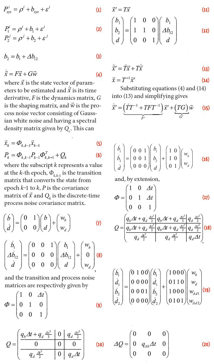
As a quick review, development of Kalman filters often starts with the continuous-time state-space system model given by
Equation 4
This can then be converted to the discrete-time equivalent which is given by
Equation 5
Equation 6
For details about the meaning/ interpretation of the above terms and equations and how they are obtained from the continuous-time equations, the reader is referred to one of the many textbooks available on Kalman filtering. Here, the focus is on how to derive models to handle the different GNSS time scales.
With this in mind, a very common clock model used for single-system GNSS is
Equation 7
where d is the receiver clock drift and, wb and wd are the process noise values for the clock bias and clock drift states, respectively. The spectral densities of the latter two terms are defined based on the quality of the receiver’s oscillator. For simplicity, we assume herein that the two process noise terms are uncorrelated, which is not true in general. However, accounting for the correlation between the two processes is well understood and can be easily added.
Starting Simple. As a starting point for the multi-system case we will, for the time being, use the substitution in equation (3) such that the state vector consists of the receiver clock bias for system one (b1), the inter-system offset between the two systems (Δb12), and a single clock drift.
Two things are worth noting at this point. First, for simplicity we are excluding any position or velocity states from the equations. From the perspective of the system model (i.e., equation (4)), the position and velocity states are unrelated with the clock states and thus can be added or removed as necessary. Of course, any practical system will include such states when processing real data, but these will only serve to complicate the discussion that follows here.
Second, by only including a single clock drift state, the model implicitly assumes that both GNSSs have the exact same frequency, which, as mentioned in the opening paragraphs, is generally not the case. We will revisit this assumption again later. Mathematically, the system model for the Kalman filter under consideration can be written as
Equation 8
Equation 9
where qb is the spectral density of the clock bias of the reference system, qd is the spectral density of the clock drift, and Δt is the time difference between epochs k and k‒1.
In other words, we treat the intersystem offset as a random constant.
Adding extra systems to this model is therefore straightforward because one need only add an extra constant to the state vector (and corresponding rows and columns of zero to the process noise matrix).
One Clock Bias Per System. As with the least-squares case, a bit more housekeeping is associated with this model because we need to first define a reference system and then keep track of what inter-system offsets are being estimated. Consequently, we prefer to estimate a “separate” clock bias for each system. To do this, we transform the state vector in equation (8) as follows:
Equation 11
Equation 12
where the second state, b2, is obtained directly from equation (3).
From equation (11), we can write the following two equations:
Equation 13
Equation 14
Equation 15
which is of the same form as equation (4) and can thus be used to derive an equivalent discrete-time Kalman filter. Doing so for the state vector in equation (12) gives
Equation 16
Equation 17
Equation 18
The peculiar thing about equation (18) is that the process noise for clock bias states is perfectly correlated. In other words, the matrix is rank-deficient. Filter designers would normally shudder at this thought since perfect correlation amongst state estimates — that is, perfect correlation within P — normally leads to numerical instabilities.
In this case, however, we are only dealing with the uncertainty added in the Kalman filter’s prediction step, not the uncertainty of the states themselves (i.e., P is still full rank because the measurements from each system still only update the clock bias for that system). In fact, the perfect correlation between the clock biases makes sense because this model was derived from the (albeit inaccurate) assumption that all system time scales have the same frequency, and thus predictions of their respective clock biases are equally uncertain.
Equations (16) to (18) are generally easier to program than equations (8) to (10) because — as with the least-squares case — a measurement from a particular system only relates to the clock bias for that system.
Back to Reality. We now return to the inaccurate assumption that all GNSS time scales have the same frequency. Fortunately, since the GNSS time scales drift with respect to each other at a very low rate — again, on the order of nanoseconds per day — the above models would likely be sufficient for relatively short processing periods.
For example, if an application processes 24 hours of data at a time, the accumulated drift between systems would be on the order of a few meters (i.e., a few nanoseconds scaled by the speed of light). If this is less than the magnitude of other errors — and the application can tolerate this level of error — then using the foregoing models probably will not adversely affect results. By extension, shorter processing runs will be even less affected.
However, what if an application requires a more rigorous model? In that case, the best approach would be to estimate a separate clock drift for each system. For the two-system case discussed earlier, the system model might look as follows:
Equation 19
where the subscript on the clock drift states denotes the system to which it applies. Also, note that each clock drift state is driven by the sum of a common process, wd, and a system-specific process, wΔdi (where i denotes the system). The common term models the receiver’s oscillator while the system-specific term models the drift of each system’s time scale (and is thus likely very small, by comparison).
The drawback of this model is that the size of the state vector increases by two for every new system used. An alternative but less rigorous approach would be to update equation (8) to model the inter-system offset (Δb12), not as a random constant, but as a random-walk process driven by a very small spectral density.
Doing this and applying the transformation in equation (12) will yield the same transition matrix as in equation (17), but the process noise matrix in equation (18) would have to be increased by the following matrix
Equation 20
where qΔb is the spectral density used to drive the intersystem bias. The net effect of matrix (20) would be to ensure that the process noise for the different clock biases are not fully correlated, thus allowing them to change more independently of each other.
Summary
This article has looked at some approaches to estimating the clock biases for the different GNSSs, with particular focus on Kalman filter models. These models will be more important in the short term because the time offsets between the various GNSSs are not readily available.
As these offsets are included in the various navigation messages, the models presented here should — theoretically, at least — degenerate to the single-system case. Of course, this assumes that the accuracy of the broadcast offsets is sufficiently high. If not, the above models may still be needed to estimate the residual offsets.