Working Papers explore the technical and scientific themes that underpin GNSS programs and applications. This regular column is coordinated by Prof. Dr.-Ing. Günter Hein, head of Europe’s Galileo Operations and Evolution.
Working Papers explore the technical and scientific themes that underpin GNSS programs and applications. This regular column is coordinated by Prof. Dr.-Ing. Günter Hein, head of Europe’s Galileo Operations and Evolution.
In GNSS receivers, the acquisition process is the first stage of the signal-processing module. It consists in assessing the presence of GNSS signals and providing a rough estimation of the incoming signal parameters: the Doppler frequency and the code delay.
To detect the presence of the signal, the received signal is correlated with a succession of locally generated replicas until the acquisition detector crosses a predefined threshold. One commonly used criterion of acquisition performance is the probability of detection when the parameters of the local replica are (close to being) correct. This probability should be as high as possible but under unfavorable conditions, such as adverse environments, detection becomes a challenge.
Initially, GNSS signals were only defined on one component (such as GPS L1 C/A) but the new generation of signals has two components (such as GPS L1C, GPS L5, Galileo E1 OS, Galileo E5 a/b, and so forth): a data component that carries the navigation message and a pilot component, which does not carry any useful information.
Designers of the modern civil signals introduced the pilot component in order to avoid the data bit transition problem during the tracking process. From the point of view of signal acquisition, however, the presence of a systematically known secondary code on the pilot component still implies bit sign transition. The presence of the pilot signal also means that the total signal power is split between components, thus impacting the way to process such a signal to gather all the signal power.
The objective of this article is to study the typical sources of performance degradations of the GNSS acquisition process that are generally overlooked in the literature and to assess their effects on the acquisition of new GNSS civil signals. We will focus on degradations due to (1) the uncertainties brought by the choice of the acquisition grid, (2) the presence of bit sign transition, and (3) the non-compensation of the code Doppler. Further to the pure acquisition performance, we also analyze the acquisition of the secondary code for new GNSS signals and the frequency refinement because these factors are necessary conditions with which to initiate standard tracking.
This study takes place in the context of the development of a GNSS software receiver that aims at acquiring any GNSS civil signals at 27 dB-Hz and higher with a strong probability of detection set to 95 percent. As a consequence, all presented results refer to this test case.
In this article, we will first introduce the required acquisition parameters to achieve the 27 dB-Hz/95 percent objective without considering any aforementioned source of degradation. Then, we discuss each point of degradation independently and analyze its effect on the probability of detection.
GNSS Signals
In this article, we consider the civil GPS and Galileo signals in the L1/E1 and L5/E5 bands.
The main points of design of a GNSS signal are:
- the carrier frequency fL
- the spreading codes c1 characterized by their length Nc1, its chipping rate fc1, or equivalently its chip duration Tc1 = 1/fc1
- the spreading code chip modulation
- the navigation message d on the data component and the secondary code c2 on the pilot component (and sometimes also on the data component).
Table 1 summarizes the main signal features for the considered GNSS signals.
The down-converted and filtered composite GNSS signal entering the correlation block of the receiver can be generically represented as follows:
s(t) = ADd(t – τ)C2,D(t – τ)c1,D(t – τ)pD(t – τ) cos(2π(fIF + fd)t + φ0,D) + Apc2,P(t – τ)C1,P(t – τ)pP(t – τ) sin(2π(fIF +fd)t + φ0,P) + n(t) (1)
where
- x stands for “D” for the data component and “P” for the pilot component
- Ax is the signal amplitude on the component and depends upon the total signal power C
- px is the subcarrier modulating the spreading codes
- τ is the receiver PRN code delay
- f1F is the received intermediate frequency of the receiver
- fd is the incoming Doppler frequency
- φ0,x is the initial phase on each component depending on the initial phase of the incoming signal
- n is the incoming noise, which is assumed to be a white noise with centered Gaussian distribution and a constant two-sided power spectral density equal to N0/2 dBW-Hz.
Note that in this expression, the role of the RF front-end equivalent filter is purposely ignored for simplification reasons.
To complete the generic expression of the received GNSS signal (1), Table 2 provides the value for each parameter. As can be seen, the GNSS L5 signals are in quadrature; however, the phase relationship between the two components of GPS L1C is not yet specified. (For details, see the article by J. W. Betz et alia listed in Additional Resources section near the end of this article.)
For the purposes of this article, we designated L1C to be an in-phase signal as is the case for Galileo E1 OS. GPS L1C presents a power difference in both components — 75 percent of the power in the pilot component and 25 percent of power in the data component — whereas the total signal power is split in half 50/50 for the other GNSS composite signals.
GNSS Acquisition Performance in Ideal Case
This section presents the acquisition process in the case when none of the sources of error mentioned in the introduction are considered which can be found in many assessment articles in the literature. As explained in the introduction, the chosen test case is to acquire any GNSS civil signals at 27 dB-Hz (total signal carrier-to-noise-density ratio or C/N0) with a probability of detection of 95 percent.
Correlation Operation. Considering the correlation operation for one component of the GNSS signal and assuming that:
- there is no data bit sign transition during the correlation process
- the correlation operation lasts for TI seconds
- the parameters of the processed signal and the local replica are constant during the correlation operation such that the code delay error ετ and the Doppler frequency error εf are constant and the carrier phase error at the beginning of the correlation process is εΦ0.
The in-phase and quadrature-phase correlator outputs can be modelled as:
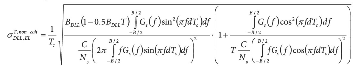
Equation (3) (see inset photo, above right, for all equations)
Note that the aforementioned correlator outputs model neglects the cross-correlation between the data and pilot component because the spreading codes were chosen to be as orthogonal as possible. Note also that the local spreading code is assumed to have the same modulation as the spreading code of the received signal.
Acquisition detector. A receiver can acquire composite GNSS signals by using correlator outputs based on one of the two components (in general, the pilot component) or both data and pilot components. In either case, the acquisition detector is defined as the sum of the squared correlator outputs (2 when only one component is used, 4 when two components are used). The acquisition detector for one component is thus
Equation (4)
where K represents the number of non-coherent summations. In this case KTI is referred to as dwell time, and the parameters of the local replica (local PRN code delay ̂τ and Doppler ̂fd) are constant for the K correlations.
The acquisition detector based on the use of two components can be easily derived accordingly.
Probability of detection. The basic principle of acquisition is to sequentially compute the acquisition detector for all possible values of local code delay and local Doppler until the detector crosses a predefined threshold Th. The set of the tested couples (̂τ, ̂fd)
is defined as the acquisition matrix, and its size depends upon the uncertainty on the incoming signal code delay and Doppler frequency and on the sampling of these uncertainties.
The tested values of the acquisition matrix are referred to as acquisition bins, and the distance between two consecutive tested values is referred to as bin size. The detection performance of such a detector is generally computed based on a hypothesis test for each visited acquisition matrix bin: hypothesis H0 assumes that the desired signal is not present and is tested against hypothesis H1 that assumes that it is present.
Under hypothesis H0 the correlator outputs only consist of independent Gaussian noises. In this case, the (normalized) detector follows a centered χ2 distribution with 2K or 4K degrees of freedom for the one-component and two-component cases, respectively. For a desired probability of false alarm Pfa, we can thus define the appropriate threshold Th.
The alternative hypothesis H1 assumes that the signal is present, meaning that the parameters of the local replica are almost aligned with the ones of the received signal. In this case, the (normalized) detector follows a non-central χ2 distribution with 2K or 4K degrees of freedom for one-component and two-component cases, respectively.
The non-central parameter of the χ2 distribution depends upon the receiver signal C/N0, the correlation duration TI, and the uncertainty of the parameters (̂τ, ̂fd)
due to the acquisition bin size. We can then compute the probability of detection Pd by comparing the detector distribution to the threshold Th. As a synthesis, the key acquisition parameters are presented in Table 3.
Minimum Dwell Time to Reach a Desired Probability of Detection. To find results related to our test case, we selected a desired probability of false alarm Pfa = 1e–3 as described in the RTCA, Inc. article referenced in Additional Resources. To reach this objective, determining the dwell time KxTI is important. As TI is generally taken equal to the spreading code period during the acquisition process, K is the critical parameter to play with.
Assuming that the acquisition bin size is infinitely small (thus meaning that ετ = εf = 0), Table 4 indicates the value of K to reach the proposed objective. This table shows that the composite GNSS signals having a data/pilot power share of 50/50 percent require a dwell time twice as short when both components are used compared to when only one component is used.
In the table, note that for GPS L1C, with a data/pilot power share of 25/75 percent, using only the pilot component or both components produces equivalent results. Finally, the well-known preferability of having a long coherent integration time to improve the acquisition detection performance explains why, for example, the GPS L1C and Galileo E1 OS require a lower dwell time than GPS L1 C/A or GPS L5. (See the discussion in F. Bastide et alia cited in Additional Resources.)
Effect of Acquisition Bin Size on Acquisition Detection Performance
Clearly, it is irrelevant to assume that the acquisition bin size is infinitely small. Indeed, a trade-off should be chosen between the acquisition bin size and the acquisition duration: a large bin size leads to degradation of the acquisition performance (the error between the tested values and the true values can be significant), while a narrow bin size means a significant number of bins potentially have to be visited, thus increasing the mean-time-to-acquire the signal.
In general, the acquisition grid is defined as a function of the maximum acceptable degradation on the detector. Following the example used in the RTCA/DO-235B, we chose
- a Doppler bin size of 1/2TI, corresponding to an equivalent degradation of the received signal C/N0 of 0.9 dB, which corresponds to a maximum Doppler frequency error |εf| ≤ 1/4TI
- a bin size in the code delay domain sufficient to generate a maximum equivalent degradation of the received signal C/N0 of 2.5 decibels. The code delay bin size thus depends on the autocorrelation function shape (and in fact on the RF front-end filter as well). For example, it corresponds to a bin size of one-half chip for an unfiltered GPS L1 C/A or GPS L5 signal.
Figure 1 shows the probability of detection as a function of the Doppler uncertainty created by the bin size for the selected test case and the number of non-coherent summations given by Table 4. In the worst case (limit of the cell), the probability of detection falls from 0.95 down to 0.8. A more relevant figure is the average probability of detection over the bin, assuming that the actual Doppler error is a random variable uniformly distributed over the entire bin. The average probability of detection is also plotted in Figure 1 and equals 0.91.
Figure 2 shows the same thing for the code delay uncertainty within one acquisition bin. In the worst location (on the edge of a bin in the acquisition grid), it goes down from 0.95 to 0.43 while the average probability of detection over the bin is 0.74.
If the worst cases in the frequency and time domains are combined, the total loss on the equivalent received C/N0 is 3.4 decibels and results in a probability of detection down to 0.25 instead of 0.95. The average probability of detection over the bin is around 0.67, thus showing a theoretical degradation of performance of 28 percent.
Bit Sign Transitions and Receiver Performance
The presence of bit sign transitions affects receiver performance in signal acquisition detection. The following discussion addresses this phenomenon and associated factors.
Bit Transition Problem. The correlator output models provided in Equation (3) assumed that the data and/or the secondary code bits are constant during the correlation interval. During the acquisition process, however, we have no reason to assume that the integration interval is aligned with the data bit. Although often neglected in the literature, it thus seems necessary to develop the correlation output model consider-ing bit sign transitions. The authors have performed such a study, including the theoretical aspects for single- and dual-component signals, and a paper — M. Foucras et alia (2014a) in Additional Resources — describing the results will be submitted for publication. The following is a short summary with corre-sponding results.
The presence of a bit sign transition during the correlation operation degrades the useful part of the correlator output without modifying the power of the noise. This results in a degradation of the acquisition detector amplitude, the nature of which will depend upon the location of the bit sign transition in the integration interval, the number of non-coherent summations, and the Doppler frequency error εf as described in the paper by C. O’Driscoll.
In particular, the expression of the non-centrality parameter in case of a bit sign transition during the integration interval is given in M. Foucras et alia (2014a). As might be expected, the worst case is for a bit sign transition occurring in the middle of the correlation interval.
For all GNSS signals discussed in this article except GPS L1 C/A, a bit sign transition can occur at each spreading code period. This means that the correlation duration should be limited to the code duration, and that even then, a bit sign transition can potentially degrade all correlator outputs. In the article by M. Foucras et alia (2014b), the authors have identified for each GNSS signal the resulting average probability of detection for the number of bit sign transitions, taking into account the probability of occurrence.
In contrast, the acquisition performance of the GPS L1 C/A signal, when considering bit sign transition, depends on the correlation duration. Indeed, because the data bit duration is 20 times longer than the spreading code period, we can use correlation durations of 1, 2, 4, 5, 10 or 20 milliseconds. Each case will have a different probability of undergoing a sign transition during the correlation. Consequently, for an equivalent dwell time — say, 20 milliseconds — the effect on the acquisition performance depends on the choice of TI as explained in M. Foucras et alia (2014b).
As shown in Figure 3, when the TI is too short, the effect of the bit sign transition is slight, but it does not allow optimal detection. On the contrary, for long TI, the effect of the bit sign transition is significant. Based on Figure 3, it appears that a correlation duration of 4 to 10 milliseconds is optimal to have the lowest dwell time to reach a probability of detection of 95 percent.
Resulting Probability of Detection. Table 4 provided the required dwell time to reach a probability of detection of 95 percent for a signal with a C/N0 of 27 dB-Hz without considering bit sign transition or uncertainty due to the acquisition bin size. For the same dwell time and C/N0, Table 5 shows the average probability of detection based on Monte Carlo simulations assuming that the distribution of the location of bit sign transition is uniform within the correlation interval (assumed equal to one spreading code). As discussed previously, for GPS L1 C/A we chose the coherent integration time to be the spreading code period (one millisecond). Note that in this latter case — considering the bit sign transition, Figure 3 showed that this value for TI is not the optimal one.
Table 5 shows that all the composite signals are highly affected, mostly due to the fact that the correlation duration has to be chosen equal to the data bit/secondary code bit duration. As a consequence, it seems necessary for these signals to use techniques that are insensitive to data bit sign transitions, such as the techniques described in the article by M. Foucras et alia (2012). These techniques are generally more demanding in terms of resources. However, GPS L1 C/A is almost not affected thanks to its structure based on a data bit duration 20 times longer than the spreading code duration.
Uncompensated Code Doppler and Receiver Performance
We now turn to the question of the effect of an uncompensated code Doppler on acquisition detection performance.
Code Doppler problem
The Doppler frequency, mainly caused by the satellite motion and the receiver local oscillator, affects the processed signal by modifying
- the central carrier frequency — a change estimated by the acquisition process
- the code frequency (chipping rate) resulting in a code Doppler fcd which depends on the incoming Doppler frequency fd, the carrier frequency fL and the chipping rate frequency fc1 according to
Equation (5)
The modification of the code frequency leads to a change in the spreading code period as can be seen in Figure 4 where three periods of a four-chip spreading code are represented:
- A positive code Doppler frequency causes the spreading code duration to shrink (Tcd < Tc1).
- A negative Doppler shift causes the spreading code duration to expand (Tcd < Tc1).
The problem of the presence of an uncompensated code Doppler resulting in a difference between the code frequency of the received and the local signals for GPS L1 C/A has been addressed by several authors. E. D. Kaplan and C. Hegarty. (See Additional Resources). Foucras et alia (2014c) showed that the degradations due to uncompensated code Doppler are even more significant for the new generation of GNSS signals (higher code frequency, lower L-band central frequency, BOC modulation).
Table 6 presents the offsets between the local and received spreading codes after the dwell time for the signals being considered in this article. For GPS L1 C/A, GPS L1C, and Galileo E1 OS, the offset is lower than one chip even for high incoming Doppler frequency. Still, the offset can sometimes be greater than one code delay bin size, which can be problematic. For L5 signals, the offset exceeds one chip for an incoming Doppler of several hundreds of hertz with the considered dwell time. For high Doppler frequencies this means that the offset is too high to provide correct acquisition performance, as it will be shown later.
To illustrate this point, Figure 5, Figure 6, Figure 7 and Figure 8 represent the deformation of the squared correlation functions between the incoming signal spreading code and the local replica spreading code for GPS L1 C/A, GPS L5, Galileo E1 OS and GPS L1C, respectively, due to uncompensated code Doppler and with the dwell times as defined in Table 4.
For BPSK-modulated signals (GPS L1 C/A and GPS L5), the shape of the autocorrelation function becomes rounded and offset compared to the reference triangular curve. The amplitude of the maximum value of the correlation function is also reduced, and the peak is shifted to the right for a negative Doppler. The result is a degradation of the probability of detection and a potential missed detection due to the motion of the correlation peak with time.
Even if the correlation function–peak offset is not such a problem for GPS L1 C/A due to its relatively slow chipping rate, this can be a real problem for GPS L5, as seen in Figure 6 where the correlation peak has moved by more than one chip over the 217-millisecond dwell time. For Galileo E1 OS, the CBOC modulation’s correlation function has a significantly reduced amplitude and its shape becomes flat when the code Doppler increases due to the presence of the side peaks. This can then create a detection problem as several bins could trigger a detection.
If the slip between the received and the local spreading codes exceeds one chip, then the correlation process no longer makes sense because the power of the signal cannot be accumulated since the correlator output is essentially noise. Figure 9 shows the linear relationship between the incoming Doppler frequency and the time to the slip of one chip.
For the maximum incoming Doppler frequency considered in this article (10 kilohertz), the slip of one chip occurs after 154 milliseconds for a GNSS signal at L1 and after only 12 milliseconds for GNSS L5 signals. For GPS L5, for example, that means the previously computed dwell time of 217 milliseconds would not be realistic as it implies a slip of 18 chips. So, the code Doppler clearly needs to be dealt with in a GPS L5 or Galileo E5a/E5b receiver, and potentially in a GPS L1 C/A, GPS L1C, or Galileo E1 OS receiver.
To complete this part of our investigation, Figure 10 presents the losses on the maximum amplitude of the squared autocorrelation function. The maximum losses are for L5/E5 signals, because these experience a slip of more than one chip (Figure 6). The minimum loss is for GPS L1 C/A (1.9 decibel for a code Doppler of 10 kilohertz), which is better than GPS L1C (2.5 decibels) and Galileo E1 OS (4.5 decibels) due to its BPSK modulation, even if the dwell time is longer (126 milliseconds instead of 50 or 80 milliseconds).
Resulting probability of detection. Let us now consider the resulting probability of detection taken in = 0 (Figure 11). Clearly, for GNSS L5 signals, the probability of detection decreases because the shift between the incoming and the local signals is too large.
Performance of the Acquisition-to-Tracking Transition
Once acquisition has been successful, the frequency estimate is on the order of a few tens or hundreds of hertz, depending upon the acquisition bin size. However, at the initiation of the tracking process, a refinement on the Doppler frequency is required in order to ensure locking the phase lock loop (PLL).
Frequency tracking. One solution is to use a frequency lock loop (FLL), which refines the estimation of the Doppler frequency. This is a critical stage in GNSS signal processing because, if this transition is not well calibrated, even a successful acquisition can lead to unsuccessful tracking, especially at low received C/N0.
The authors undertook a performance study for various FLL schemes, which was described in the article by M. Foucras et alia (2014d) listed in Additional Resources. Based on the proposed test case, the probability of achieving FLL lock was analyzed assuming a C/N0 of 27 dB-Hz. The four FLL discriminators examined in the study are the cross-product (CP), the decision directed cross product (DDCP), the differential arctangent (Atan), and the four-quadrant arctangent (Atan2). We should mention that during this initial phase of GNSS signal tracking being studied, bit synchronization has not yet been achieved.
Table 7 summarizes the expressions, linear regions, and characteristics of the four candidate FLL discriminators. As only two discriminators are bit sign–transition insensitive, this feature plays a key role in the choice of the discriminator for the best FLL scheme.
Probability of Successful Transition. The key figure of merit for the acquisition-to-tracking process is the probability of successful transition (or convergence) of the FLL, regardless of the initial frequency error after acquisition (within the correct acquisition bin, thus with a Doppler error within
Equation (6)
hertz in the proposed case) as a function of the GNSS signal and the FLL discriminator. The convergence is assessed by making sure that the loop is locked after 20 seconds of tracking. The probabilities are obtained based on 200 runs per configuration.
For the simulations, the article by M. Foucras et alia (2014d) (Additional Resources) showed that it is better to choose an FLL loop bandwidth BL that is relatively reduced even though this reduces the response time of the loop. BL = 1 Hz is used in the following results.
Finally, for composite GNSS signals, two techniques were investigated: the first one consists of tracking only the pilot component and the second one consists of tracking both components by computing a FLL discriminator based on an average of the data and pilot discriminators (thus using the whole available signal power).
Two figures present the probabilities of successful transition for a signal with a C/N0 equal to 27 dB-Hz. Figure 12 considers the pilot-only cases whereas Figure 13 considers a scheme using the total available power. As expected, successful convergence depends upon the initial frequency error (it is better to start close to the correct value).
In the legend of each figure, the mean probability of successful transition in the cell is provided. As can be observed, for GPS L1 C/A, whatever the Doppler initial frequency error, the FLL always converges using the CP or Atan2 discriminators, thus finely dealing with bit sign transitions.
- For GNSS composite signals, however, this is no longer the case:
- For the GPS L1C signal, due to the presence of 75 percent of the signal power contained in the pilot component, the difference between the two schemes (considering pilot or both components) is slight. The performance for both bit transition–insensitive discriminators is similar and around 0.95 in mean value.
For Galileo composite signals, it appears preferable to use both components. In this case, for the Galileo E1 OS signal, the average value is 0.94 for the DDCP discriminator and has a performance very similar to GPS L1C. For the Galileo E5a or Galileo E5b signals (and GPS L5, not shown here), the probabilities to get locked are very low (mean value 0.23), which constitutes a significant problem for the acquisition-to-tracking transition. This can be explained by the short integration time (one millisecond) associated to these signals which implies a high correlator output noise variance for a signal with a C/N0 equal to only 27 dB-Hz.
Secondary code acquisition performance. The pilot component was initially introduced to avoid the data bit transition problem on the data component. Indeed, the pilot component is free of transition once the secondary code is demodulated. This leads to the use of longer coherent integration for a more robust tracking.
In an article by M. Foucras et alia (2013), the authors provided a detailed analysis on the probability of acquiring the secondary code for several GNSS composite signals. The main conclusion of this study was that the C/N0 threshold to acquire the secondary code with a very high probability was much lower than 27 dB-Hz and should not be a problem.
Conclusions
Signal acquisition is a crucial processing step in GNSS receivers. A useful signal must be extracted from the incoming signal that is assimilated in the background RF noise, and its parameters should be estimated. Due to these conditions, the acquisition process at low received C/N0 is a challenge.
We conducted a detailed analysis of all the sources of acquisition degradations, treating each point separately as described in this article, to understand its specific effect. Our emphasis was on the probability of detection, voluntarily putting aside the time-to-acquire factor, which is operationally of equivalent importance. The article also concentrated on a specific test case, which was to be able to acquire a GNSS signal with a received C/N0 of 27 dB-Hz with a probability of detection of 95 percent.
The first point that we addressed was the degradation of signal acquisition performance caused by the estimated parameters’ uncertainty brought by the size of the acquisition bin. A typical bin size results in an average degradation of the probability of detection on the order of 5 to 20 percent in the test case that we considered.
We then showed that the problem of the bit-sign transition was not a big issue for the acquisition of GPS L1 C/A. This is because a data bit transition can occur only every 20 spreading code periods, and a good choice of the coherent integration time enables a receiver to limit the degradation of acquisition performance.
However, for the new GNSS signals considered in our research, a bit sign (data or secondary code) transition can occur at each spreading code period, and the adverse effect on the acquisition performance can become substantial. As a consequence, we highly recommend use of a transition-insensitive acquisition technique for these signals even if they are more computationally expensive.
We also showed that an uncompensated code Doppler particularly affects the acquisition performance for GNSS L5 signals due to their high frequency chipping rate. If not taken care of properly, this effect results in a correlation function shape becoming rounded and flattened, leading to a potentially poor estimation of the incoming code delay.
Our research also showed that the BOC-based signals are more influenced by code Doppler due to the shape of their correlation function. As a consequence, if code Doppler is not taken into account by the receiver, it becomes necessary to limit the acquisition dwell time even if this penalizes the acquisition performance at low C/N0 (it does anyway).
Finally, we described the use of FLL for the carrier acquisition-to-tracking process, with the main conclusions being to use bit transition–insensitive discriminators for composite GNSS signals.
Additional Resources
[1] Bastide, F., and O. Julien, C. Macabiau, and B. Roturier, “Analysis of L5/E5 Acquisition, Tracking and Data Demodulation Thresholds,” in Proceedings of the 15th International Technical Meeting of the Satellite Division of The Institute of Navigation (ION GPS 2002), Portland, Oregon, USA, 2002, pp. 2196 – 2207
[2] Betz, J. W., and M. A. Blanco, C. R. Cahn, P. A. Dafesh, C. J. Hegarty, K. W. Hudnut, V. Kasemsri, R. Keegan, K. Kovach, L. S. Lenahan, H. H. Ma, J. J. Rushanan, D. Sklar, T. A. Stansell, C. C. Wang, and S. K. Yi, “Description of the L1C Signal,” in Proceedings of the 19th International Technical Meeting of the Satellite Division of The Institute of Navigation (ION GNSS 2006), Fort Worth, Texas, USA, 2006, pp. 2080 – 2091
[3] Curran, J. T., “Weak Signal Digital GNSS Tracking Algorithms,” Ph.D. thesis, National University of Ireland, Cork, 2010
[4] Foucras, M., (2012) O. Julien, C. Macabiau, and B. Ekambi, “A Novel Computationally Efficient Galileo E1 OS Acquisition Method for GNSS Software Receiver,” in Proceedings of the 25th International Technical Meeting of The Satellite Division of the Institute of Navigation (ION GNSS 2012), Nashville, TN, USA, 2012, pp. 365 – 383
[5] Foucras, M., (2013) and O. Julien, C. Macabiau, and B. Ekambi, “Probability of Secondary Code Acquisition for Multi-Component GNSS Signals,” in Proceedings of the 6th European Workshop on GNSS Signals and Signal Processing (SIGNALS 2013), Neubiberg, Germany, 2013
[6] Foucras, M., (2014a) O. Julien, C. Macabiau, B. Ekambi, and F. Bacard, “Probability of Detection for GNSS Signals with Sign Transitions,” IEEE Transactions in Aerospace Electronic Systems, submitted July 2014
[7] Foucras, M., (2014b) O. Julien, C. Macabiau, B. Ekambi, and F. Bacard, “Optimal GNSS Acquisition Parameters when Considering Bit Transi-tions,” in Proceedings of IEEE/ION PLANS 2014, Monterey, CA, USA, 2014
[8] Foucras, M., (2014c) O. Julien, C. Macabiau, and B. Ekambi, “Detailed Analysis of the Impact of the Code Doppler on the Acquisition Perfor-mance of New GNSS Signals,” in Proceedings of the 2014 International Technical Meeting of The Institute of Navigation, San Diego, CA, USA, 2014, pp. 513 – 524
[9] Foucras, M., (2014d) and U. Ngayap, J. Y. Li, O. Julien, C. Macabiau, and B. Ekambi, “Performance Study of FLL Schemes for a Successful Acquisition-to-Tracking Transition,” in Proceedings of IEEE/ION PLANS 2014, Monterey, California, USA, 2014.
[10] Jiao, X., and J. Wang, and X. Li, “High Sensitivity GPS Acquisition Algorithm Based on Code Doppler Compensation,” in IEEE 11th International Conference on Signal Processing (ICSP), Beijing, China, 2012, pp. 241 – 245
[11] Kaplan, E. D., and C. Hegarty, Understanding GPS: Principles and Applications, 2nd edition, Artech House, 2005
[12] O’Driscoll, C., “Performance Analysis of the Parallel Acquisition of Weak GPS Signals,” Ph.D. thesis, National University of Ireland, 2007
[13] Parkinson, B. W., and J. J. Spilker, Global Positioning System: Theory and Applications, Progress in Astronautics and Aeronautics, Vol. I, 1996
[14] Psiaki, M. L., “Block Acquisition of Weak GPS Signals in a Software Receiver,” in Proceedings of the 14th International Technical Meeting of the Satellite Division of The Institute of Navigation (ION GPS 2001), Salt Lake City, UT, USA, 2001, pp. 2838 – 2850
[15] RTCA, Inc., “Assessment of Radio Frequency Interference Relevant to the GNSS L1 Frequency Band RTCA/DO-235B.” 13-Mar-2008
[16] Van Diggelen, F. S. T., A-GPS: Assisted GPS, GNSS, and SBAS, GNSS Technology and Applications Series. Artech House, 2009
(̂τ, ̂fd)