Unmanned aerial vehicles or UAVs comprise a category of aircraft that fly without a human operator onboard. They are more popularly referred to by the misleading moniker “drones,” which masks the wide variety in their design and capability.
Unmanned aerial vehicles or UAVs comprise a category of aircraft that fly without a human operator onboard. They are more popularly referred to by the misleading moniker “drones,” which masks the wide variety in their design and capability.
UAVs can be flown autonomously or piloted remotely (in the latter case, sometimes being referred to as RPVs or remotely piloted vehicles) and span a wide range in size and complexity. The largest UAVs weigh several thousand pounds and have wingspans on the order of 100 feet. At the other end of the size and capability spectrum are the small UAVs or micro aerial vehicles MAVs). These can be as small as a large insect or a hummingbird and may be disposable.
The utility of such vehicles in military and law enforcement application is clear and will not be discussed further here. Although not as obvious, a compelling economic and social case can be made for many civilian applications of UAVs, such as environmental monitoring, forestry surveys, precision agriculture, and transportation infrastructure inspection.
A civilian application that has not received as much attention, and is the focus of this article, is avionics development and testing. Developing and certifying avionics intended for use in the safety-critical application of guiding, navigating, and controlling manned aircraft is an expensive and time consuming endeavor, due, in part, to the need to show that credible fault modes are extremely unlikely.
For designing navigation systems, this may involve collecting a large amount of data to characterize or bound tail events that have low very low probabilities of occurring. In the design of control systems, engineers may need to show that the system will continue to maintain the aircraft in a safe flying condition in the face of all credible fault modes. Evaluating some of these fault modes may require placing the aircraft in untested flight states that can be potentially unsafe.
In view of these challenges, some have investigated whether UAVs can be used as surrogate platforms for evaluating new avionics concepts and the effect this has on the overall research, development, and certification process. Precedents exist for using unmanned aircraft in this way. A case in point is NASA Langley’s AirSTAR program, which relied upon a UAV that was a dynamically scaled version of a generic, modern jet transport aircraft. Other cases include NASA Dryden’s X-48 and X-56 projects. In these situations, UAVs are used to develop control laws that would have been too dangerous to test on manned aircraft.
For example, one AirSTAR program objective required researchers to evaluate control strategies to recover from a flight upset that put an airplane in an unsafe attitude. Program managers considered manned flight tests in these angle-of-attack and sideslip angle regimes to be unsafe, but thought that candidate designs could be evaluated effectively in a UAV. The third author of this article, while at NASA Dryden, was part of the efforts that also employed UAVs to test novel, GPS-based methods for air data system calibration that hold promise for reducing the cost and effort required to calibrate these sensors, which are crucial for the safe operation of an aircraft.
The laboratory used by the University of Minnesota UAV Research Group (UMN-URG) is exploring such applications — increasing the efficiency of research, development, testing, and certification of advanced avionics concepts. In a two-part article we will provide an overview of this effort, describing the infrastructure that has been developed and used at the University of Minnesota to support this work.
In this first part, we will give a high-level description of the overall infrastructure that has been developed for the UAV lab and how it is used. This includes the flight platforms and research avionics employed by the UAV Lab. Part two of the article — to be published in the May/June issue of Inside GNSS — will present examples of current projects under way in the lab that have the potential to transform the methods used in avionics development and testing. More details about the various aspects of the system described here can be found at the University of Minnesota UAV Research Group (UMN-URG) website.
Enabling Infrastructure
Flexibility is the key to being able to use UAVs for research, where novel sensors and algorithms are often integrated. By flexibility we mean the ability to quickly reconfigure the guidance, navigation, and control (GNC) system of an aircraft. It also requires that one has access to a very accurate “ground truth” against which to measure the performance of novel and new GNC algorithms.
To accomplish this, the system developed by UMN-URG relies on four integrated components: aerial vehicles, avionics and sensors, simulations and flight software, and flight operations.
First, a fleet of test vehicles supports research experiments with respect to a variety of airframe sizes and payload requirements. Second, an avionics and sensor array supports fundamental flight sensing and communication needs, as well as specific research experiments. Third, an open source, modular simulation and software infrastructure supports experiment design, testing, and flight code development. Fourth, a set of flight operations ensures the safety and reliability of the entire flight test system while adhering to the regulatory requirements set by the FAA. Each of these components is described in detail in the following sections.
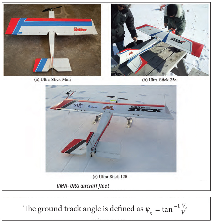
Aerial Vehicles. The current UMNURG fleet includes three versions of conventional fixed-wing aircraft that belong to the Ultra Stick family (see inset photo, above right). The Ultra Stick family is a commercially available group of radio-controlled (R/C) aircraft. Each airframe is modified to fit and carry the necessary avionics and sensors.
The Ultra Stick 120 is the largest and heaviest airframe, with a 1.92-meter wing span and 7.4-kilogram mass capable of carrying the most payload, and is equipped with the largest array of sensors. The Ultra Stick 25e is a 66-percent scale version of the Ultra Stick 120, with a 1.27-meter wing span and 1.9-kilogram mass. It serves as the primary flight test vehicle in the UMN-URG aircraft fleet due to its convenient size and is equipped with a core avionics and sensor array.
The Ultra Stick Mini is a 52 percent scale version of the Ultra Stick 120, with a 0.98–meter wing span. This aircraft is used as a wind tunnel model and is not equipped with any flight avionics or sensors. The accompanying photo shows an example of each airframe version currently operating in the fleet.
All three vehicles are conventional fixed-wing airframes with aileron, rudder, elevator, and flap control surfaces. Control surfaces are actuated by means of electric servos, with a maximum deflection of 25 degrees in each direction. The propulsion systems consist of electric motors (with varying power depending on the airframe size) that drive fixed-pitch propellers.
The aircraft systems are battery powered, designed to allow for approximately 30 minutes of power on a single charge. Table 1 presents some of the key physical properties of the three Ultra Stick aircraft operated by the UMN-URG.
Thrust for the vehicles is generated by electric outrunner brushless DC motors, which require electronic speed controllers. Actro 40-4 motors power the Ultra Stick 120 vehicles accompanied by Castle Creations ICE2 HV80 speed controllers. These motors require two 5S 5000 mAh lithium polymer (LiPo) batteries in series. A single 3S 2650 mAh LiPo battery powers the avionics and servos.
The Ultra Stick 25e vehicles incorporate Eflite Power 25 motors along with Castle Creations ICE LITE 50 speed controllers. These motors require a single 3S 3300 mAh LiPo battery. The avionics and servos are powered by the same battery as the Ultra Stick 120 avionics.
The Ultra Stick 120 was initially used as a low-cost flight test platform at NASA Langley Research Center. Aerodynamic modeling efforts have included extensive static wind tunnel tests, which were later complemented with dynamic wind tunnel tests. This was used to develop a high-fidelity model (equations of motion) of the aircraft, which NASA made publicly available. This makes the Ultra Stick 120 an ideal platform for control and model-aided navigation system research.
Unfortunately, the Ultra Stick 120 model airframe is currently out of production. To ensure the continuity of the Ultra Stick 120 as a flight test vehicle, the UMN-URG has acquired a stock of several spare airframes.
UMN-URG co-developed the Ultra Stick 25e as a flight test platform along with researchers at the Budapest University of Technology and Economics in Hungary. Over time, the needs of the two groups have evolved, and, hence, the vehicles are currently equipped with different avionics and sensors. However, the similarity in airframes allows for cooperation in critical research areas, such as control and navigation. The aerodynamic model for this vehicle was developed through flight testing at the University of Minnesota.
We use the Ultra Stick Mini primarily as a wind tunnel model. It serves as an educational tool for undergraduate courses and laboratories for the Department of Aerospace Engineering & Mechanics (AEM), for example, to derive basic aerodynamic coefficients from wind tunnel data.
GNC Avionics. Figure 1 shows the architecture of the core system (both airborne and ground based) used to fly our aerial platforms. This hardware combination is installed onboard each Ultra Stick 120 and 25e airframe and represents the minimum requirement for research experiment flight tests. Some individual airframes have additional sensors to support specific experimental functions. We will highlight these specific sensor outfits following a description of the core system.
At the center of the avionics and sensor array is the flight computer, a 32-bit PowerPC microcontroller with a clock frequency of 400 megahertz and 760 MIPS of processing power that performs floating-point computation. The flight computer utilizes a real-time operating system called eCos, with the flight software written in C; although autocoded Simulink can be used as well.
The flight software is modularized with standard interfaces, allowing different modules (e.g., different control or fault detection algorithms) to be easily interchanged. We will present more details on the software architecture later in this article. The current software uses about two percent of CPU capacity and runs at a framerate of 50 hertz.
The flight computer has a wide range of input-output (I/O) capabilities. It supports communication with external devices via TTL and RS232 serial, SPI, I2C, and Ethernet. Communication with servo actuators is handled with pulse width modulation (PWM).
Flight data is recorded at 50 hertz, stored in the 64 MB SRAM available onboard, and downloaded after each flight via Ethernet connection to a ground station laptop. The Ethernet connection is also used to load flight software onto the flight computer. The flight computer is mounted on an interface board, which is a custom design and handles power and the communication interface with external devices.
A failsafe board is used to switch control of the aircraft between manual mode (human remote-control or R/C pilot stick-to-surface operation) and flight computer automatic mode. In both modes, pilot commands are recorded and provided to the flight computer. This enables the option for piloted closed-loop control or signal augmentation experiments. Telemetry is sent to a ground station laptop through a wireless radio at 10 hertz. The transmitted data is visualized on a custom developed synthetic heads-up display (HUD). The HUD provides real-time information about attitude, altitude, airspeed, and GPS performance.
In addition to the flight computer and mode switch, each flight test vehicle is equipped with a core set of onboard sensors. Measurements of static and dynamic air pressure from a Pitot probe are used to estimate airspeed and altitude. Pressure transducers communicate with the flight computer over inter-integrated circuit (I2C) bus.
Angular rates and translational accelerations are measured with an inertial measurement unit (IMU), which communicates through serial peripheral interface (SPI) bus. This sensor has an accelerometer triad, a gyroscope triad, and a magnetometer triad. Finally, a GPS receiver provides position and velocity information at one hertz and communicates over a TTL serial line.
The interface board is a custom design from the UMN-Twin Cities Department of Aerospace Engineering and Mechanics. A table in the Manufacturers section near the end of this article summarizes the components in the core avionics and sensor array, which have a total cost of $2,780. This array is integrated into a single module, shown in Figure 2, that we call the Goldy flight control system (FCS), which is common to all flight test vehicles.
Several vehicles are equipped with additional sensors to enhance their research capabilities. An Ultra Stick 120, named Ibis, and an Ultra Stick 25e, named Thor, are equipped with five-hole Pitot probes. Each Pitot probe takes four additional air pressure measurements along with the standard pitot tube measurement. The additional measurements are used to estimate angle-of-attack and sideslip angle.
Ibis also inherits from NASA Langley the wingtip sensor booms that measure angle-of-attack and sideslip angle directly. To better suit navigation research, it is also equipped with two additional GPS antenna/receiver systems, control surface deflection sensors, and a camera mount on the fuselage.
Flight Operations
Typical UAV flight experiments are divided into three segments: take-off, research experiments, and landing. Each flight begins with a manual take-off by the R/C pilot. For safety, flight operations require winds below 10 mph with no gusts.
Once airborne, the pilot flies the aircraft into a racetrack pattern with constant altitude (below 400 feet) and obtains a steady trim. The racetrack pattern is generally used to maximize available straight and level flight time. Dimensions of the pattern are defined by line-of-sight requirements. In an emergency, the pilot must always be able to visually guide the aircraft back to safe operation. As a result of these safety constraints, the Ultra Stick 120 and 25e can only achieve about a 20-second maximum of straight and level flight.
UMN-URG has applied for and received certificates of authorization (COAs) from the Federal Aviation Administration (FAA) to operate both of its conventional aircraft at the UMN UMore Park facility. UMore Park is a 5,000-acre university- owned property located near Rosemount, Minnesota, consisting of research agriculture fields.
In obtaining the COAs, we have found that it is indispensable to learn from groups that have gone through the application. In this regard, UMN-URG was fortunate to have the help of Professor Eric Frew, director of the Research and Engineering Center for Unmanned Vehicles at the University of Colorado at Boulder.
There, UMN researchers operate UAVs within a small, 0.28-nauticalmile– radius section of this facility centered around a 3,000 by 100-foot turf runway with airspace up to 400 feet above ground level (AGL). To operate legally within this airspace, the UMN UAV Research Lab has published operational and emergency procedures, crew duty requirements, and maintenance plans. Maintenance procedures, airframe status, and pilot currency are tracked. The operations team consists of at least two certified pilots, with Class II flight physicals, acting as pilotin- command (PIC) and an observer to see and avoid traffic.
UMN researchers notify the FAA prior to operating within the COA airspace so that the agency can include these planned activities in Notices to Airmen (NOTAMS) in order for manned aircraft to avoid low-altitude flights in the area during UAV flight tests. Although these procedures and plans may seem daunting, once they are in place, applying for a COA is a relatively straightforward process, and the FAA is very helpful at guiding organizations through the necessary steps.
Simulation Environment
A simulation environment provides an important complement to the flight test system. Simulation-based development and validation prior to flight testing reduces the total design cycle time for experimental research algorithms. The UMN-URG maintains three simulations, illustrated by the block diagram in Figure 3.
A common Matlab/Simulink implementation of the aircraft dynamics is shared between the three simulations. This shared implementation includes flight dynamics, actuator models, sensor models, and an environmental model. All experimental research algorithms must pass through a validation test in each simulation before consideration for flight testing.
The lowest-level and most basic simulation allows for control algorithms to be implemented in Simulink, a block diagram environment for multidomain simulation and model-based design. This frequently serves as a first step in the design process of new control algorithms.
The mid-level simulation is a software-in-the-loop (SIL) simulation. The SIL simulation allows a research algorithm, written as flight code in C and interfaced via S-function, to be validated in Simulink.
Finally, the highest level simulation is a hardware-in-the- loop (HIL) exercise. This simulation allows a research algorithm, written as flight code in C and implemented on the Goldy FCS, to be interfaced with Simulink and validated. These simulations are available open source to facilitate collaboration and promote common development platform among researchers around the world. The latest versions of all three simulations can be downloaded as a package from the UMN-URG website.
Nonlinear Simulation. We have implemented a six-degree-of- freedom (6-DOF) nonlinear simulation model of the aircraft dynamics in Simulink. This model represents a set of conventional rigid-body equations of motion for generic fixed-wing aircraft. Forces and moments due to aerodynamics, propulsion, and the environment are integrated numerically to solve the nonlinear differential equations.
The environmental model includes a detailed model of Earth’s atmosphere, gravity, magnetic field, wind, and turbulence. Models of the aircraft subsystems, such as actuators and sensors, are also included.
Each test vehicle is associated with three simulation components: physical properties, a propulsion model, and an aerodynamic model. This allows the nonlinear simulation model to be easily reconfigured for a particular test vehicle. Physical properties for each airframe are determined in the lab, where moments of inertia are found using bifilar pendulum swing tests. We use wind tunnel tests to characterize the motor and propeller thrust, torque, and power for each aircraft.
The aerodynamic models vary depending on the airframe. The Ultra Stick 120 aerodynamic model is derived from extensive wind tunnel data obtained at NASA Langley Research Center. This high-fidelity model covers large ranges of angle-of-attack and angle-of-sideslip aerodynamics and is implemented as a look-up table. The Ultra Stick 25e aerodynamic model is derived using flight test data and frequency domain system identification techniques, as described in the article by A. Dorobantu et alia cited in the Additional References section at the end of this article. This model is linear and assumes constant aerodynamic coefficients. The Ultra Stick Mini aerodynamic model is based strictly on wind tunnel data obtained by the UMN-URG.
Linear models of the aircraft dynamics (about an operating point) are frequently desired for the design of control algorithms. The 6-DOF nonlinear simulation model is set up for trimming and linearization. The simulation package provides automatic functions to perform these tasks. After verifying the performance of a typical control algorithm using the linearized dynamics, it must again be verified using the nonlinear simulation. The gray-shaded controller shown in Figure 3 illustrates this verification process.
Software-in-the-Loop. The SIL simulation uses the 6-DOF nonlinear simulation model in feedback with a control algorithm implemented as flight code in C. This implementation of the control algorithm is interfaced with Simulink through an S-function block. Figure 3 represents the SIL simulation with the blue-shaded controller. The flight control algorithm alone is linked to the S-function; the remainder of the flight software is not included.
The primary purpose of the SIL simulation is to verify the accuracy of a control algorithm transition from Simulink (mathematical discrete-time model) to flight code written in C.
Hardware-in-the-Loop Simulation. The HIL simulation is an extension of SIL simulation that includes the flight software and flight computer. Figure 3 represented this simulation environment as the red-shaded controller.
The entire flight software suite is compiled and runs on the flight computer in sync with the nonlinear simulation model. The MathWorks Real-Time Windows Target toolbox is used to ensure the simulation runs in real-time on a Windows PC. This is crucial for obtaining meaningful results when the flight computer is included in the simulation loop.
The nonlinear simulation model, in Simulink, interfaces with the flight computer using a serial connection. The flight software is modified in two ways in order to interface correctly with the HIL simulation. First, the data acquisition code (which normally solicits the onboard sensors) reads sensor data from the nonlinear simulation. Second, the actuator commands (which are normally delivered to the actuators via PWM signals) are sent back to the nonlinear simulation.
Through the HIL verification process, any implementation issues or bugs associated with a control algorithm are identified and resolved. The HIL simulation is also useful in testing attitude and navigation state estimation algorithms, such as the one described in a later section, Navigation.
The HIL simulation provides an interface for an R/C pilot through a USB R/C-style remote. The aircraft state can be visualized via FlightGear, which is an open-source flight simulator. Researchers can use this interface to evaluate the performance and handling qualities of a control algorithm prior to flight testing.
Flight Software
The software implemented on the flight computer is programmed as a single-thread, real-time process executing at 50 hertz. A version control and documentation management system manages the entire real-time software suite and simulation environment described in the previous section.
Real-Time Software. The flight software is divided into code modules that are called in sequence by the main function. Each module is dedicated to a certain type of computation, for example, attitude/navigation estimation or control algorithm. All candidate modules use an interface layer, which allows the software engineer to easily select which modules to compile in order to build the full program. In general, each type of module must be present in the compiled code, even if no computation native to a given module type is required. Figure 4 shows a schedule and order diagram of the code modules implemented in the flight software.
A real-time clock is managed by a free, open-source, real-time operating system (RTOS) called eCos. The RTOS provides alarms to the flight software that trigger code modules to execute. Three alarms are scheduled and validated in order to allow enough time for the software to execute on a 0.02-second frame.
The first alarm triggers the data acquisition module (DAQ) immediately at the start of a new frame. This module reads data from the onboard sensors. For the HIL simulation, a different DAQ module is compiled in order to interface with Simulink.
An INS/GPS algorithm is executed in the navigation filter module (NAV). The guidance law module (GL) generates commands to the control system. Potential sensor faults, such as biases, can be added in the sensor fault module (SF).
The main control algorithm (CL) is computed next. Signals required for system identification (SI) can be augmented after the control law. Potential surface faults can be added in the surface fault module (SF). Once this sequence of modules has executed, the software waits for the next alarm.
The second eCos alarm triggers the actuator module (ACT), which sends PWM signals to the actuators. Once again, for HIL simulation a different ACT module was compiled in order to interface with Simulink.
Maintaining a consistent time in between the DAQ and ACT modules is important; it represents the time delay of the flight computer. After the ACT module has executed, the software waits for the next alarm.
A third eCos alarm allows the data logging (DL) and telemetry (TM) modules to execute. The sequence of modules then repeats as the software waits for the DAQ alarm from eCos, which indicates the start of a new frame.
The flight software is built and compiled using a Makefile that specifies which version of each code module is included in the program. For example, to compile software for HIL simulation instead of flight, the HIL versions of DAQ and ACT are selected in the Makefile. This approach allows for modularity and software flexibility.
Version Control. The flight software and simulation environments are managed by a version control program. The UMN-URG uses a subversion (SVN) server to manage a software development repository. This repository is available publicly on the research group website.
The flight software is automatically documented using Doxygen, a utility that allows documentation to be generated directly from source code. Each file in the flight software suite has a special Doxygen header that enables generation of the automatic documentation.
Navigation
The attitude state of an aircraft must be estimated from measurements provided by the onboard sensors. On the other hand, we can measure position and velocity states directly with a GPS receiver.
Typical receivers, however, do not provide data at a sufficiently high rate for use in feedback control of aircraft. For example, the GPS receiver used by the UMN-URG provides data to the flight computer at one hertz. Consequently, our UAV avionics requires a sensor fusion algorithm to provide accurate and high bandwidth estimates of the aircraft attitude, position, and velocity. These are known as the navigation states.
The navigation state estimates are computed using an algorithm that integrates an inertial navigation system (INS) with GPS. More in-depth description of INS/GPS integration can be found in the navigation literature; so, all we will provide here is a high level description of the system. An INS provides measurements at higher bandwidth than a typical GPS receiver. For example, the IMU used by the UMN UAVURG provides measurements at 800 hertz. Due to flight software limitations, however, the flight computer only samples the IMU at 50 hertz.
Numerically integrating IMU measurements to obtain the navigation state estimates leads to unbounded errors that grow over time. A combined INS/GPS algorithm provides a solution that has the high bandwidth of the INS and the drift-free long-term stability of the GPS measurement.
Attitude can be equivalently described by Euler angles or the quaternion. The INS/GPS estimation algorithm uses the quaternion for computation and converts the solution to Euler angles for control.
Attitude determination using an IMU calls for integrating the angular velocity measurement ωB to propagate the attitude forward in time. Rate gyroscopes measure inertial rotation and should be compensated to account for the Earth’s rotation rate and the transport rate due to the Earth’s curvature. For consumer/automotive IMUs used in low-cost UAV applications such as the Goldy FCS, however, these terms are small compared to the noise level in the sensors, and are thus ignored.
The INS uses measurement of the acceleration to generate position and velocity estimates. A triad of accelerometers in the IMU provides measurement of the specific force fB acting on the aircraft. When the IMU is rigidly attached to the aircraft, this specific force is measured in the body frame and therefore needs to be rotated into the navigation frame before integration and propagation in time. This rotation uses the aircraft attitude to formulate the required transformation matrix CNB. CNB transforms the accelerometer output from the body frame (B) to the NED frame (N).
After compensating for gravity and the Coriolis effect, the force can be integrated once to yield velocity and twice to yield position. Figure 5 presents a block diagram of the structure of the INS/GPS integration algorithm.
An extended Kalman filter (EKF) is used to correct the attitude, velocity, and position estimates for errors. In order to improve the navigation solution between GPS measurements, and to allow coasting during short GPS outages, the EKF makes frequent corrections to compensate for the inertial sensor errors.
Although more sophisticated sensor error models exist, we use a simplified, single-bias-per-sensor error model. This model is robust to parameters that are unobservable when the UAV is not accelerating. Using this model, the estimated sensor bias not only represents the true bias corrupting the measurement, but also accounts for all unmodeled errors that corrupt the sensor measurement.
The INS/GPS algorithm is initialized as soon as a valid GPS measurement becomes available (when implemented estimates are initialized at the first available position and velocity measurements. Because the initialization is set to occur on the ground before a flight test begins, the attitude is initialized to an approximate attitude of the aircraft on the ground. Figure 6 presents a portion of navigation flight data obtained during a fligt test with Thor.
The flight test result in Figure 5 shows the navigation solution (computed in real-time onboard the aircraft) along with GPS measurements as markers. The INS/GPS integration algorithm connects the GPS measurements with a smooth, high bandwidth position estimate.
Innovations in the position estimate from the EKF are small (typically below two meters for position, and 0.5 m/s for velocity), which indicates convergence in the algorithm. Although this flight test was conducted with an Ultra Stick 25e test vehicle, numerous data sets exist in the SVN record of Ultra Stick 120 flight tests that validate the same attitude and navigation algorithm. These data sets are publicly available for download here.
Baseline Flight Control Design
The platform requires a simple and reliable baseline control algorithm as a benchmark. We designed and validated a classical controller for each vehicle through simulation and flight tests. This controller serves as the standard for any experiment that requires closed-loop control.
The design has a two-tiered structure: an inner-loop attitude controller and an outer-loop flight management system. The inner-loop controller tracks desired pitch and roll angles of the aircraft while damping out oscillations present in the open-loop dynamics. The outer-loop controller maintains desired altitude, airspeed, and heading direction. The outerloop controller is built around the inner-loop controller.
Inner-Loop Controller. The inner-loop attitude controller tracks desired pitch and roll angles while damping oscillations in the open-loop dynamics. The desired closed-loop rise times are one second, and the overshoot is no greater than five percent. The closed-loop is robust and has gain margin greater than ±6 decibels and phase margin in excess of 45 degrees.
Although the inner-loop control architecture is common for the entire fleet of test vehicles, the gains are tuned individually in order to account for variations in the aircraft dynamics. One set of gains is valid for the Ultra Stick 25e and another for the Ultra Stick 120.
For the control design, the nonlinear simulation model is linearized about a trim condition for each vehicle. Trim conditions are defined as level flight at 17 m/s and 23 m/s for the 25e and 120 models, respectively. The linearized dynamics are decoupled into longitudinal and lateral/directional subsystems; inner-loop controllers are designed separately.
The longitudinal controller is shown in Figure 7, where “AC (lon)” is the linearized aircraft model. The inputs to the model are throttle setting (δthr) and elevator deflection (δe). The outputs used in feedback are pitch angle (θ) and pitch rate (q).
A proportional gain pitch rate damper (Kq) is applied to increase damping. The pitch angle–tracking controller (Kθ) uses proportional-integral gain. Integrator anti-windup logic (A/W) is implemented to handle actuator saturation. The inputs to the closed-loop system are pitch angle reference (θref) and δthr (throttle not controlled).
Figure 8 illustrates the lateral/directional controller, where “AC (lat/dir)” represents the linearized aircraft model. The inputs to the model are aileron (δa) and rudder (δr) deflections. The outputs used in feedback are roll angle (ϕ), roll rate (p), and yaw rate (r).
A proportional gain roll rate damper (Kp) is applied to reject disturbances in turbulent conditions, while a proportional gain yaw damper (Kr) is implemented to increase damping in the Dutch roll mode. The controller also requires a washout filter to avoid an adverse yaw effect during turns. The roll angle–tracking controller (Kϕ) uses proportional-integral gain; A/W logic handles actuator saturation. The resulting input to the closed-loop system is roll angle reference (ϕref).
The validated the performance of the combined inner-loop controller using simulation and flight tests. The test scenario was a step reference pattern of various amplitudes and lengths. Pitch axis commands were applied independently from roll axis commands.
We used this type of pattern in order to excite the closed-loop dynamics over a broad frequency range. Simulation and flight tests confirmed that the controller, which was designed using a linear model, performed as expected both in the simulation and in flight. Figure 9 shows the combined flight test and SIL simulation results for Thor.
The flight test results confirm that the inner-loop attitude tracking controller objectives are satisfied. The rise times for the pitch and roll axes are around one second, the pitch response displays a five percent overshoot, and no overshoot appears in the roll response. Strong agreement between the flight data and the simulation result affirms the accuracy of the aircraft model and the reliability of the controller.
Outer-Loop Controller. The outer-loop controller is a flight management system that tracks altitude, airspeed, and ground track angle. Its characteristics include no overshoot on the ground track angle, and maintaining altitude and airspeed within ±5 meters and ±2 m/s, respectively. Figure 10 shows the architecture.
Inputs to the inner-loop control system are throttle setting (δthr), pitch angle reference (θref), and roll angle reference (ϕref). The outputs employed for outer-loop control are the indicated airspeed (V), altitude (h), and ground track angle (ψg). The ground track angle is defined as: (see inset photo, above right, for equation), where Ve and Vn are the east and north velocities estimated by the navigation filter.
The three guidance blocks shown on the left side of Figure 10 provide the flight management system with commands Vref, href, and ψg,ref. The altitude controller (Kh) produces a pitch angle reference command, and the airspeed controller (KV) produces a throttle command.
Although not ideal for engine-out scenarios, this architecture was selected for simplicity. Both Kh and KV use proportional-integral control and implement integrator A/W logic (not shown in Figure 10) in order to safely limit the commands provided to the inner-loop control system. The throttle command is constrained between 0 and 1, and the pitch angle reference is constrained to 20 degrees.
The ground track angle controller (Kψg) uses proportional gain, and, hence, the roll angle reference ϕref can be constrained directly at ±45 degrees. This limiting is required to prevent the aircraft from rolling over due to large ground track angle step commands.
A flight test was conducted with Thor to verify the performance of its flight management system. The test consisted of a series of 90-degree ground track–angle step commands. In the absence of wind, this should result in a square pattern. In the presence of wind, the airplane flies a rectangular pattern that drifts in the direction of the wind.
Figure 11 compares flight data with a SIL simulation of the ground track angle, airspeed, and altitude signals throughout the maneuver.
The simulation and flight test results confirm that the outer-loop flight management system satisfies our objectives. The ground track angle is followed by the aircraft, while altitude is held within ±5 meter and airspeed, within ±1.5 m/s. Figure 12 overlays a visualization of the aircraft trajectory on a satellite image of the test flight area.
In Figure 12, a rectangular trajectory reflecting the presence of wind begins at the origin. Using the flight data, an estimate of wind direction and speed is obtained by examining the drift. We applied the estimated wind components in the nonlinear simulation, which shows strong agreement with the flight test.
Conclusion
The aerospace community needs to continue developing flexible and efficient flight test platforms to support the testing and validation of new theory. The University of Minnesota operates such a platform with advanced research capabilities in control, guidance, navigation, and fault detection. The hardware, software, and simulation infrastructure of this platform, as well as the flight data from UMN-URG flight tests, are available open-source at the group’s website for the benefits of the entire research community.
Collaborating with researchers, using this open-source infrastructure, and flight testing with these platforms will expedite the development and application of new theory that could one day revolutionize aerospace technology.
Acknowledgments
This research was partially supported under the NASA Langley contract NNH077ZEA001N entitled “Analytical Validation Tools for Safety Critical Systems,’’ NASA Langley contract NNX08AC65A entitled “Fault Diagnosis, Prognosis and Reliable Flight Envelope Assessment,’’ NASA STTR subcontract NNX12CB02C from Tao Systems Inc. entitled “Robust Aeroservoelastic Control Utilizing Physics-Based Aerodynamic Sensing,’’ and National Science Foundation (NSF) Grant No. NSF-CNS-0931931 entitled “CPS: Embedded Fault Detection for Low-Cost, Safety-Critical Systems.’’ Any opinions, findings, conclusions, or recommendations are those of the authors and do not necessarily reflect the views of NASA or the NSF. The article is based on a paper presented at the 2013 American Controls Conference (ACC), held June 17–19, 2013, in Washington, DC.
Additional Resources
[1] Bauer, P., and J. Bokor, “Tuning and Improvements in a Waypoint and Trajectory Tracking Algorithm,” in AIAA Guidance, Navigation, and Control Conference, no. 2012-4604, Minneapolis, Minnesota USA, 2012
[2] Chu, C-C., and F. A. Lie, and D. Gebre-Egziabher, “Dual Hypothesis Filter for Robust INS/Camera Fusion,” Proceedings of Institute of Navigation International Technical Meeting, San Diego, California USA, January 2013
[3] Chu, C-C., and F. A. Lie, L. Lemay, and D. Gebre- Egziabher, “Performance Comparison of Tight and Loose INS-Camera Integration,” in Proceedings of the 24th International Technical Meeting of the Satellite Division of the Institute of Navigation (ION GNSS 2011), Portland, Oregon USA, 2011
[4] Dorobantu, A., and A. Murch, B. Mettler, and G. Balas, “Frequency Domain System Identification for a Small, Low-Cost, Fixed-Wing UAV,” AIAA Journal of Aircraft, Vol. 50, No. 4, pp. 1117-1130, July, 2013
[5] Freeman, P., “Robust fault detection for commercial transport air data probes,” Master’s thesis, University of Minnesota, November 2011
[6] Freeman, P., and R. Pandita, N. Srivastava, G. Balas, “Model-based and Data-driven Fault Detection Performance for a small UAV,” IEEE/ ASME Transactions on Mechatronics, Vol. 18, No. 4, pp. 1300-1309, 2013
[7] Freeman, P., and P. Seiler and G. Balas, “Robust Fault Detection for Commercial Transport Air Data Probes,” in IFAC18th World Congress, Milan, Italy, pp. 13723-13728, August 2011
[8] Gebre-Egziabher, D., and B. Taylor, “Impact and Mitigation of GPS-Unavailability on Small UAV Navigation, Guidance, and Control,” Report #2012-2, University of Minnesota, Department of Aerospace Engineering and Mechanics, November 2012
[9] Jordan, T., and J. Foster, R. Bailey, and C. Belcastro, “AirSTAR: A UAV Platform for Flight Dynamics and Flight Control System Testing,” Proceedings of 25th AIAA Aerodynamic Measurement Technology and Ground Testing Conference, no. 2006-3307, San Francisco, California USA, 2006
[10] Koifman, M., and I. Y. Bar-Itzhack, “Inertial Navigation System Aided by Aircraft Dynamics,” IEEE Transactions on Control Systems Technology, Vol. 7, pp. 487-493, July 1999
[11] Koifman, M., and S. J. Merhav, “Autonomously aided strapdown attitude reference system,” AIAA Journal of Guidance, Control, and Dynamics, Vol. 14, No. 6, pp. 1164-1172, 1990
[12] Lie, F. A., and D. Gebre-Egziabher, “Synthetic Airdata System,” AIAA Journal of Aircraft, Vol. 50, No. 4, pp.1234-1249, July, 2013
[13] Owens, D. B., and D. E. Cox and E.A. Morelli, “Development of a Low-Cost Sub-Scale Aircraft for Flight Research: The FASER Project,” in 25th AIAA Aerodynamic Measurement Technology and Ground Testing Conference, no. 2006-3306, San Francisco, California USA, 2006
[14] Pandita, R., Dynamic Flight Envelope Assessment with Flight Safety Applications. Ph.D. thesis, University of Minnesota, 2010
[15] Pandita, R., and J. Bokor and G. Balas, “Closed-loop performance metrics for fault detection and isolation and controller interaction,” International Journal of Robust and Nonlinear Control, 2011