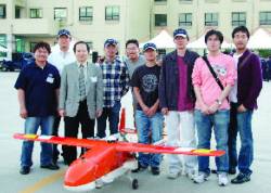
 SNUGL team members: From left to right, Byungjoon Park (BJ Hobby Craft), Jihoon Kim, Prof. Changdon Kee, Am Cho, Bosung Kim, Dongkeon Kim, Noha Park, Sanghoon Jeon, and Donghwan Bae
GPS has been widely used as a navigation sensor for numerous applications including unmanned aerial vehicles (UAVs). Many researchers have devoted considerable efforts to expand the role of GPS in guidance, navigation and control to determining an aircraft’s attitude. That would enable us to use a GPS receiver as a sensor for an automatic control system as well as a navigation sensor.
GPS has been widely used as a navigation sensor for numerous applications including unmanned aerial vehicles (UAVs). Many researchers have devoted considerable efforts to expand the role of GPS in guidance, navigation and control to determining an aircraft’s attitude. That would enable us to use a GPS receiver as a sensor for an automatic control system as well as a navigation sensor.
However, most GPS-based attitude determination algorithms have used multiple antennas and corresponding signal-tracking modules, which incur relatively high capital costs. In a 1998 paper, R. P. Kornfeld and coauthors suggested an efficient algorithm that enables attitude determination with only single-antenna GPS. (See Additional Resource section near the end of this article.) They also demonstrated the feasibility of an autopilot system that relied on single-antenna GPS–based attitude with a human pilot in the loop as a controller.
With this motivation and goal, Seoul National University GNSS Lab (SNUGL) developed an automatic flight control system for a UAV based on a single-antenna GPS. SNUGL has conducted many flight tests using such a system and developed a variety of related applications since it undertook the first flight in 2000.
In 2003, SNUGL succeeded in waypoint path following control and, in 2005, located the position of a ground target — both achieved by means of a single-antenna GPS–guided UAV. Furthermore, the SNUGL team enhanced the single-antenna GPS–based attitude determination method and developed a method to estimate wind and calibrate airspeed sensor using a single-antenna GPS receiver and airspeed sensor.
More recently, the team also successfully demonstrated fully automatic control of the UAV from takeoff to landing using a single-antenna GPS receiver, and subsequently first prize in the Korean robot aircraft competition consecutively in 2007 and 2008.
This article describes the system development and recent flight tests that validated this design.
Single-Antenna Attitude Determination
The SNUGL method synthesizes the aircraft attitude, which is called pseudo-attitude, from single-antenna GPS velocity measurements using a simple point mass aircraft model assuming conditions of coordinated flight. Under that assumption, the lift acceleration vector (l) is equal to the vector difference of normal components of the aircraft acceleration vector (an) and the gravitational acceleration vector (gn) perpendicular to the velocity vector.
This approach estimates the aircraft acceleration vector from GPS velocity measurements using Kalman filtering. Then the “pseudo-roll” angle (Φ) is determined geometrically as the complementary angle to the angle (δ) between the horizontal ground plane (P) and the estimated lift acceleration vector. Figure 1 illustrates the vectors used to compute pseudo-roll angle.
Pseudo-attitude can be obtained in another way by introducing a new body frame. This approach provides a basis for designing our full-state estimator and controller. The x-axis of the new body frame coincides with the aircraft velocity vector. The z-axis is defined as the opposite direction of the normal component of the specific force perpendicular to the velocity vector. Then the new body frame coincides with the wind frame in coordinate flight without wind.
To calculate pseudo-attitude, we can decompose the direction cosine matrix that represents the coordinate transform from a NED (north, east, down) frame to the new body frame, using the following equations:
Euler Angle Rate and Body Angular Rate. The Euler angle rates are obtained by filtering pseudo Euler angles; we determine the body angular rates from the coordinate transformation. Because the x-axis of the body frame is defined as the aircraft velocity vector, the body-axis components of the velocity vector are determined as shown by Equation 4.
From the foregoing results, we constituted a single-antenna GPS estimator that consists of three kinematic filters and an attitude synthesizer. It generates full states of a UAV from GPS position and velocity measurements.
Satellite Visibility. Because the proposed flight control system is based on the navigation solution of only a single-antenna GPS receiver (Figure 2), the minimum number of visible satellites and available signals is important for continuity of the system.
Figure 3 uses sample daily broadcast GPS ephemerides to analyze the number of satellites that would be in view during various flight maneuvers over an area that corresponds to the middle latitudes. The analysis shows that a single-antenna GPS receiver would be sufficient here for use as a main sensor because minimally four visible satellites are guaranteed at sharp turns with roll angles of up to 60 degrees.
Controller Design
To design linear full-state feedback controllers, we adopted the linear quadratic regulator (LQR) control laws to provide practical feedback gains, since LQR is known to provide the optimal performance and makes it possible to combine stability augmentation and autopilot system. We computed the optimal gain matrix from linearized lateral and longitudinal equations using MATLAB.
As shown in Figure 4, control inputs consist of two parts: feedforward and feedback control. Feedforward values are open-loop inputs calculated from the output commands, whereas feedback values are closed-loop inputs calculated from the tracking errors and control gain.
A UAV is assumed to follow a concatenation of steady-state trajectories under a coordinated-flight condition. The output commands consist of total velocity (VT), vertical flight path angle(γ), and yaw (Ψ) based on a given steady-state trajectory as shown in Equation 5.
They decide the trim values of state variables as Equation 6. U, V and W denote the forward, sideward, and downward velocities of an aircraft. P, Q, and R are, respectfully, roll, pitch, and yaw body angular rates. Φ, Θ, and Ψ are roll, pitch and yaw angles. Rt,cmd is the turn radius of the-circle-to-be-followed. The subscript 1 denotes the trim value.
We can calculate trim inputs in two other ways: one is numerical computation from dynamic equations using specified output commands, the climb-rate, and coordinated flight constraints, and the other is experimental flight tests. By using these trim inputs as feedforward inputs, the problems of tracking the concatenated steady-state flight trajectories
are much simplified.
The error states, which are heading error (ψ), cross track error (y) and altitude error (h), are not related to the trim conditions and do not affect the trim inputs. They are defined as the deviations from the commanded values, and how we compute them depends on the output commands, such as altitude (Vt,cmd, Hcmd), heading (Ψcmd), and path control.
Figure 5 shows error states for helical path control. They are the deviations from the commanded values of the intersection point between the path and the radial vertical plane passing through the current aircraft position (PE,PN) shown in Equation 7.
The longitudinal controllers include climb-rate, altitude, and glide slope controllers, whereas the lateral controllers include bank, heading, line track, and circle track controllers. Table 1 and Table 2 show the output (or control) commands and state and input vectors for longitudinal and lateral controllers.
Automatic Takeoff and Landing
The automatic takeoff controller includes a runway track controller and a climb-out controller. The runway track controller maintains UAV alignment with the runway centerline.
During rolling, a process is added to prevent the rollover of the UAV. The climb-out controller controls the climb rate using the elevator with full throttle. The lift off is decided from airspeed and climb rate. The UAV completes climb-out when it achieves a pre-specified altitude and an altitude controller begins operation.
Airspeed, pitch, and altitude are controlled in the flare mode. The linearized equation of motions and output vectors for a flare controller is shown in Equation 8.
Because the number of outputs exceeds the number of controls, the flare controller determines the input that produces the smallest output-error–minimizing performance index. Thus, appropriate output commands need to be activated for the smooth touchdown.
We decided these commands through simulation and flight tests. In simulation and flight test, during flare, we found that elevator input oscillates with the period of short-period mode. Note that single-antenna GPS–based estimator does not provide true pitch; the pseudo-pitch is in fact a vertical flight-path angle. We solved this oscillation by applying a low-pass filter to an elevator input. The time constant of the filter was set to the short-period mode.
System Configuration
We developed an automatic flight control system for flight tests. The most salient feature of the system is that it uses a single-antenna GPS receiver as the main sensor for an unmanned aerial vehicle (UAV).
Although one can control a UAV automatically by using only a single-antenna GPS receiver in a stand-alone mode, automatic landing requires more accurate position information; thus, they use differential GPS (DGPS), in which the GPS receiver in the UAV requires DGPS corrections to eliminate common errors in GPS pseudoranges.
Figure 6 shows the whole control system, which is composed of a ground station segment and a UAV segment. Ground station equipment consists of laptop computers, a wireless modem, a GPS receiver for the DGPS reference station, an R/C (radio control) transmitter, and an electric power system. UAV equipment include a PC/104 stack, a single-antenna GPS receiver, a wireless modem, a PWM (pulse-width modulation) processing board, an R/C receiver, a set of batteries, and a MEMS inertial measurement unit only for data recording (Figure 7).
Commercial off-the-shelf (COTS) PC/104 modules are adopted as a flight control computer. The maximum output rate of the used GPS receiver is 10 Hz and it is the same as the update rate of both the estimator and controller. The UAV for flight tests is a fixed-wing, twin tail-boom, pusher-type aircraft with a gasoline-powered propeller engine. It has a wingspan of 2.5 meters and a gross weight of about 13 kilograms including payloads.
The programming environment for both onboard and ground computers is Microsoft Windows 2000/XP professional and Visual C++ with MFC (Microsoft Foundation Class Library). Windows OS is not a real-time OS, but is good enough for verifying the automatic flight control system. Data communications between programs onboard or between programs in ground computers are achieved through Ethernet network by using UDP (User Datagram Protocol). Onboard and ground computers communicate through wireless modems by using RS232 serial communications.
Figure 8: Real-time flight monitoring program
Figure 9: 3D Trajectory of Flight Test
Flight Test Results
The main sensor of the UAV is a single-antenna GPS receiver. In order to show its full potential, no inertial sensors, such as gyros and accelerometers, are incorporated into the system. Instead, the single-antenna GPS–based estimator estimates full states of the UAV. To improve the robustness to wind effects, the GPS-derived forward velocity of the UAV was replaced by the airspeed measured from the Pitot tube.
The single-antenna GPS estimator starts to estimate attitude information when the UAV velocity reaches more than the pre-specified value of three meters per second. The UAV exceeds this velocity shortly after it starts to move.
When the UAV rolls on the runway, the controller handles the steering at the same time. However, experiments showed that rudder control was more effective when the UAV accelerated. During takeoff, the system activates the heading controller and climb-rate controller were activated with full throttle power.
After the UAV reaches the designated altitude, it uses the waypoint path controller. We employed line and circle track controllers for linear and circular horizontal paths.
Vertical path control has two modes: altitude control and vertical slope track control, with the latter mode used for glide slope control.
Integrators are designed to eliminate the steady-state errors on the velocity and position tracking errors. The aircraft speed is maintained at around 26 m/s except for takeoff and landing. Flare control uses forward speed/pitch/altitude.
Figure 10 and Figure 11 show, respectively, horizontal and vertical trajectories of fully automatic control of the UAV from takeoff to landing. (Commanded paths are dotted lines.) The UAV starts to roll along the runway at point A and takes off shortly after. When the altitude reaches 70 meters, the UAV has a smooth transition interval of three seconds.
At point B, the waypoint path controller is activated. After that, the UAV starts to descend at point C, following a curved glide slope approach path with a glide slope angle of three degrees. Finally, the UAV performs flare control at point D and then touches down on the runway. The UAV conducted this flight using only a single command. Weather conditions included a wind of two to three m/s at the ground level.
Figure 12 shows that actual trajectories in the linear glide slope path converged well to the command path due to the effects of integrators. Horizontal cross track errors converge up to three to four meters, and vertical slope track errors converge up to a half meter.
During three flight tests, ground levels of touch-down points varied by one meter due to the limit of DGPS vertical positioning accuracy as shown in Figure 13. However, this problem was overcome by careful design of the flare control system, such as including appropriate output commands and saturation. A low-cost ultrasonic altimeter or carrier-phase DGPS might be helpful to decide flare and touchdown altitude.
Conclusions and Future Work
This article described the methods of designing an estimator and controllers in order to use a single-antenna GPS receiver as a primary sensor for a UAV system without use of inertial sensors. We implemented differential GPS to obtain high accuracy position information for path control, including curved approach and automatic landing.
To improve the robustness to wind effects, the forward velocity of the UAV uses airspeed measurements from a Pitot tube. Flight test results show that the proposed automatic controller can operate successfully using only a single-antenna GPS receiver and airspeed sensor. A primary factor of concern identified during the efforts described in this article is longitudinal control; therefore, more tuning of the control system could improve the lateral performance.
Our results indicate that a single-antenna GPS receiver can be used as a main sensor for a flight control system of an expensive UAV. Also, such a low cost system (as low as $50) can be a backup system for a general aviation aircraft and a high cost UAV including Global Hawk and Predator. In future work, we will apply a wind estimation algorithm to improve the robustness to various wind conditions.
Acknowledgements
The authors thank the late Sanghyo Lee for his early contribution of the flight tests, and Youngsoo Cho (Electronics and Telecom. Research Institute), Subong Sohn, Bhoram Lee, Noha Park, Donghwan Bae (Samsung Electronics), Heunggyo Cheong (Samsung Engineering), Sujin Choi (Korea Aerospace Research Institute), Bosung Kim (Air Transportation Lab., Georgia Tech.), Dongkeon Kim (SK Telecom), and Joonsol Song (Seoul National University), for all their contributions to this research. Dr. Doyoon Kim (Defense Acquisition Program Administration) is also acknowledged for reviewing and editing this article.
Additional Resources
[1] Cho, A., and J. Kim, S. Lee and C. Kee, “Wind Estimation and Airspeed Calibration Using the UAV with a Single-Antenna GNSS Receiver and Pitot Tube,” IEEE Transactions on Aerospace and Electronic systems, accepted for publication, 2009
[2] Kornfeld, R. P. (1998), and R. J. Hansman, and J. J. Deyst, “Single-Antenna GPS-Based Aircraft Attitude Determination,” Journal of the Institute of Navigation, vol.45, Spring 1998, pp.51-60.
[3] Kornfeld, R. P. (2001), and R. J. Hansman, J. J. Deyst, Keith Amonlirdviman and E. M. Walker, “Applications of Global Positioning System Velocity-Based Attitude Information,” Journal of Guidance, Control, and Dynamics, vol. 24, No. 5, 2001.
[4] Lee, S., and J. Kim, A. Cho, H. Cheong and C. Kee, “Developing an automatic control system of unmanned aircraft with a single-antenna GPS receiver,” in Proc. ION GNSS 2004, Sep. 2004.
[5] Park, S., and C. Kee, “Enhanced method for single-antenna GPS-based attitude determination”, Aircraft Engineering and Aerospace Technology, vol. 78, no. 3, 2006.
[6] Sohn, S., and B. Lee, J. Kim, and C. Kee, “Real-time Target Localization Using a Gimbal Camera for a Single-antenna GPS-based UAV,” IEEE Transactions on Aerospace and Electronic Systems, vol. 44, issue 4, pp. 1391-1401, 2008.